마이크로소프트 엑셀에서 동적 데이터를 정렬하는 방법은 무엇입니까?
재고 기록과 같이 끊임없이 변화하는 데이터 세트를 관리할 때, 정보를 효율적으로 정렬하는 것은 정확한 보고와 신속한 분석에 필수적입니다. 하지만 데이터가 업데이트될 때마다 수동으로 다시 정렬하는 것은 시간이 많이 걸릴 뿐만 아니라 오류 발생 가능성이 큽니다. 그렇다면, 수량 조정이나 새로운 항목 추가와 같은 기본 데이터가 변경될 때마다 정렬된 결과가 최신 정보를 즉시 반영할 수 있도록, 엑셀 목록을 자동으로 정렬하려면 어떻게 해야 할까요?
이 문서에서는 엑셀에서 동적 데이터를 자동으로 정렬하기 위한 몇 가지 실용적인 방법을 상세히 설명합니다. 공식 기반 접근 방식, VBA 자동화 및 데이터가 변할 때 표를 계속 정렬해주는 최신 엑셀 도구들을 배우게 됩니다. 이러한 방법들은 재고 관리, 판매 추적, 성적 평가 또는 실시간 정렬된 데이터가 중요한 모든 작업에 적합합니다.
➤ 수식을 사용하여 엑셀에서 동적 데이터 정렬하기
➤ 워크시트 변경 이벤트(VBA)를 사용하여 데이터를 자동으로 정렬하기
➤ 더 쉬운 정렬을 위해 엑셀 테이블(“표 형식으로 서식 지정”) 사용하기
➤ SORT 또는 SORTBY 동적 배열 함수를 사용하여 정렬하기 (Excel365/2019+)

수식을 사용하여 엑셀에서 동적 데이터 정렬하기
이 방법은 모든 최신 버전의 엑셀에서 작동하며 원본 테이블 옆에 자동으로 업데이트되는 정렬된 데이터 복사본을 유지하고자 할 때 가장 적합합니다. 이 접근법은 순위를 부여하고 해당 순위에 따라 값을 조회하는 방식에 의존하며, 입력값이 변경됨에 따라 정렬된 테이블도 최신 상태로 유지됩니다.
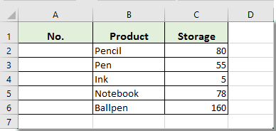
예를 들어, 여러 종류의 문구류 품목들의 재고 저장량을 관리한다고 가정해봅시다. 어떤 수량 변경이라도 즉시 반영하고 저장량을 기준으로 내림차순으로 제품을 표시하려면 다음 단계를 따르세요:
1. 원본 데이터 세트의 시작 부분에 새 열을 삽입하세요. 예제 시나리오에서는 아래 그림과 같이 원본 데이터 앞에 “번호”라는 제목의 열을 삽입하세요:
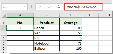
2. 셀 A2(“번호” 아래의 맨 위 셀, 데이터 범위가 A2:C6이라고 가정)에 다음 수식을 입력하여 각 제품의 저장 수량을 기준으로 순위를 계산하세요. 이를 통해 엑셀은 저장 필드를 사용하여 각 항목에 고유한 순서를 부여합니다:
=RANK(C2, C$2:C$6)수식을 입력한 후 Enter를 누르세요. RANK 함수는 C2의 저장 값과 전체 범위 C2:C6을 비교하여 순위 번호를 할당합니다(1이 가장 높은 저장량). 5개 이상의 항목이 있는 경우 C6을 필요한 범위만큼 조정하세요.
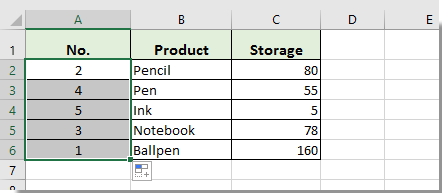
3. 셀 A2를 선택한 상태에서 채우기 핸들을 A6까지(또는 데이터의 마지막 행까지) 드래그하여 리스트의 모든 항목에 순위 수식을 적용하세요.
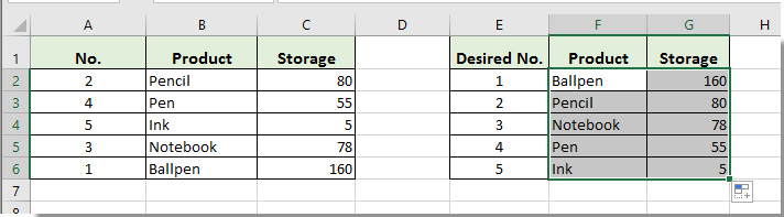
4. 동적으로 정렬된 표를 만들기 위해 먼저 원본 데이터의 헤더 행을 복사하여 새로운 위치(예: E1:G1)에 붙여넣습니다. 새로운 “원하는 번호” 열(E2:E6 예시)에 순위(1, 2, 3, …)와 일치하는 순차적인 숫자 목록을 입력하세요. 이 순서는 검색을 위한 순서를 설정합니다.
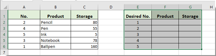
5. 새 표의 F2 셀(“상품” 옆)에 주어진 순위 번호에 해당하는 상품 이름을 검색하는 다음 VLOOKUP 수식을 입력한 후 Enter를 누르세요:
=VLOOKUP(E2, A$2:C$6, 2, FALSE)이 수식은 A열에서 주어진 순위를 검색하고 두 번째 열에서 연관된 상품 이름을 반환합니다.

6. F2에서 F6까지 채우기 핸들을 드래그하여 모든 상품 이름을 채우세요. 정렬된 저장 수량을 채우기 위해 F2:F6을 선택한 다음 G2:G6으로 채우기 핸들을 오른쪽으로 드래그하세요.
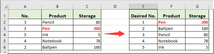
새로운 표는 저장량을 기준으로 내림차순으로 상품을 표시하며, 원본 표의 변경 사항을 항상 반영합니다:
예를 들어, 문구점에 납품이 도착했고 원래 목록에서 “펜”의 저장량을 55에서 200으로 업데이트했다면, 정렬된 표는 즉시 펜 항목을 새로운 순위와 수량으로 재배치합니다 — 수동 정렬이 필요 없습니다. 이 솔루션은 목록 관리를 자동화하여 수동 오류를 줄이고 주요 보고서를 정확하게 유지합니다.
참고:
- 중복 값(동률): 저장량에 동률이 있을 경우, 간단한
RANK는 여러 행에 동일한 순위를 부여하고VLOOKUP은 첫 번째 일치 항목만 반환합니다. 안정적인 순서를 위해 2단계를 A2에서 다음과 같은 동률 처리 수식으로 대체하세요(그런 다음 아래로 채우기):
=RANK(C2, C$2:C$6) + COUNTIF($C$2:C2, C2) - 1C$2:C$6, A$2:C$6)를 리스트가 커짐에 따라 조정하세요. 소스를 엑셀 테이블로 변환하면 유지 관리가 간단해집니다(구조화된 참조).팁:
- Microsoft 365 / 엑셀 2019+에서는 더 직접적인 동적 정렬을 위해
SORT/SORTBY를 고려하세요. - 보조 열을 피하고 싶다면, 고급 대안으로
INDEX/MATCH(또는XLOOKUP)과SMALL/ROW를 결합하여 정렬된 목록을 생성할 수 있지만, 이는 읽기 어렵고 유지 관리하기 어려울 수 있습니다.
팁 & 문제 해결: 원래 목록 크기가 변경될 때 새 항목이나 삭제된 항목이 모두 포함되도록 수식 범위를 다시 확인하세요. 목록을 확장하는 경우 참조(C$2:C$10 대신 C$2:C$6)를 조정해야 할 수도 있습니다. 자주 목록 크기가 변경되는 경우, 데이터를 엑셀 테이블로 변환하고 셀 범위 대신 테이블 열 이름을 참조하세요.
워크시트 변경 이벤트(VBA)를 사용하여 데이터를 자동으로 정렬하기
이 솔루션은 원본 표를 그대로 정렬된 상태로 유지하고자 할 때 유용합니다 — 사용자가 수정하거나 새 항목을 입력할 때마다 즉시 행이 재정렬됩니다. 이는 수동 정렬을 줄이고 공유 목록, 재고 로그 및 기타 자주 업데이트되는 기록에 잘 작동합니다.
장점: 소스 데이터를 항상 정렬된 상태로 유지; 별도의 표나 복사 없음; 모든 열 개수에 적용 가능.
단점: 매크로가 필요; 파일을 수정하는 모든 사람이 매크로 활성화된 엑셀이 필요함.
예제 시나리오: 문구점이 표에서 재고를 추적합니다. 누군가가 저장량을 변경할 때마다 해당 행이 자동으로 적절한 순위로 이동합니다.
주의해서 사용하세요: 이 방법은 데이터 레이아웃에 직접 영향을 미칩니다 — 필요한 경우 백업 또는 버전 관리를 유지하세요.
구현 방법:
1. 자동 정렬하려는 시트 탭을 마우스 오른쪽 버튼으로 클릭하고 코드 보기(View Code)를 선택하세요.
2. 워크시트의 코드 창(표준 모듈이 아님)에 다음 코드를 붙여넣으세요:
Private Sub Worksheet_Change(ByVal Target As Range)
    On Error Resume Next
    Dim SortRange As Range
    ' Adjust your range as appropriate (example: A1:C6 includes headers)
    Set SortRange = Range("A1:C6")
    ' Sort by Storage in descending order (assuming Storage is in column C)
    SortRange.Sort Key1:=SortRange.Columns(3), Order1:=xlDescending, Header:=xlYes
End Sub
3. VBA 편집기를 닫습니다. 이제 A1:C6 내의 데이터가 수정될 때마다 엑셀은 “저장” 열(C열)을 기준으로 내림차순으로 전체 범위를 자동으로 다시 정렬합니다.
참고:
Range("A1:C6")을 실제 테이블(헤더 포함)에 맞게 업데이트하세요.- 이 매크로는 표준 모듈이 아닌 워크시트 모듈(예: Sheet1 (Code))에 있어야 합니다.
- 매크로가 실행되지 않으면 자동 정렬이 작동하지 않으므로, 통합 문서를
.xlsm로 저장하고 매크로가 활성화되어 있는지 확인하세요.
팁:
- 다른 열을 기준으로 정렬하려면
Columns(3)인수를 원하는 인덱스로 변경하세요. - 오름차순이 필요한 경우
Order1:=xlDescending을xlAscending으로 변경하세요. - 범위가 커지는 경우, 주기적으로 고정된 주소(예:
A1:C1000)를 확장하거나 범위를 엑셀 테이블로 변환하고 매크로를 테이블 주소로 업데이트하세요.
파라미터 설명 및 문제 해결: 매크로는 선택한 열을 기준으로 고정된 범위를 정렬하며, 헤더 행이 있다고 가정합니다. 정렬이 되지 않는다면, 매크로가 활성화되어 있고 코드가 올바른 시트 모듈에 있는지 확인하세요. 사용자가 지정된 범위 외부에서 편집하는 경우, 정렬이 트리거되지 않습니다 — 모든 편집 가능한 행을 포함하도록 범위를 조정하세요.
엑셀 테이블(“표 형식으로 서식 지정”)을 사용하여 더 쉽게 정렬하기
Format as Table 기능을 사용하여 데이터 범위를 공식적인 엑셀 테이블로 변환하면 목록 관리 및 정렬에 여러 가지 이점을 제공합니다.
✅ 장점: 데이터를 추가하거나 편집할 때 구조화된 참조가 자동으로 업데이트되고, 각 열에 대한 정렬/필터링 드롭다운을 제공합니다. 열 헤더 드롭다운을 클릭하면 전체 테이블을 즉시 정렬할 수 있습니다. 새 행을 추가하면 테이블이 자동으로 확장됩니다.
⚠️ 단점: 정렬이 완전히 자동이 아닙니다 — 변경 후에도 다시 정렬하려면 클릭해야 합니다, 자동으로 정렬을 트리거하기 위해 VBA 매크로를 추가하지 않는 한 말입니다.
일반적인 시나리오: 협업 통합 문서 또는 대규모 데이터 세트에서 사용자가 시각적 조직과 빠른 행 삽입이 필요한 경우, 엑셀 테이블은 정기적인 정렬을 더 쉽고 오류를 줄일 수 있게 만듭니다.
사용 방법:
- 데이터 범위를 선택하고 Ctrl + T를 눌러 엑셀 테이블로 변환하세요. 데이터에 헤더가 있는지 확인하세요.
- 정렬하려는 열(예: 저장)의 헤더 드롭다운 화살표를 클릭하고 가장 큰 값부터 가장 작은 값으로 정렬 또는 가장 작은 값부터 가장 큰 값으로 정렬을 선택하세요.
테이블이 편집될 때마다 정렬이 자동으로 이루어지도록 하려면, 앞서 설명한 대로 VBA 매크로를 테이블이 포함된 시트에 첨부하세요. 이렇게 하면 엑셀 테이블의 쉬운 구조와 VBA 자동화가 결합됩니다.
💡 팁: 엑셀 테이블은 수식에서 구조화된 참조를 지원하므로, 데이터가 증가함에 따라 읽고 유지 관리하기가 더 쉬워집니다. 정렬을 취소하려면 열 드롭다운에서 정렬 취소를 선택하세요. VBA를 사용하는 경우, 매크로가 올바른 테이블 이름(예: ListObjects("Table1"))을 참조하는지 확인하세요.
SORT 또는 SORTBY 동적 배열 함수를 사용하여 정렬하기 (엑셀 365/2019+)
최신 버전의 엑셀(엑셀 365, 엑셀 2019 이후)에는 원본 데이터의 정렬된 버전을 실시간으로 자동 생성할 수 있는 동적 배열 함수가 도입되었습니다 — 보조 열이나 VBA가 필요 없습니다.
✅ 장점: 진정한 실시간 자동 정렬. 수식은 원본 목록이 증감함에 따라 인접한 셀로 결과를 “분출”합니다. 설정이 매우 간단합니다.
⚠️ 단점: 최신 엑셀 버전에서만 사용 가능합니다. 출력은 별도의 복사본이며, 원본 범위는 재정렬되지 않습니다.
예제 시나리오: 대시보드 표시나 보고 목적으로 실시간으로 업데이트되는 정렬된 재고 목록 사본을 원하지만, 편집 또는 데이터 입력을 위해 입력 순서를 유지하려는 경우입니다.
사용 방법:
원본 데이터 테이블이 A2:C6 범위에 있고 A1:C1에 헤더가 있다고 가정해 봅시다. 저장량을 기준으로 내림차순으로 동적으로 정렬된 테이블을 생성하려면, E2와 같은 아무 비어있는 셀에 다음 수식을 입력하세요:
=SORT(A2:C6, 3, -1)이것은 원본 테이블의 새로운 자동 정렬된 버전을 생성하며, 세 번째 열(저장량)을 기준으로 내림차순으로 정렬됩니다. 내림차순은 -1, 오름차순은 1을 사용하세요.
보조 키 또는 사용자 정의 기준 등 더 세밀한 정렬을 위해서는 SORTBY를 사용하세요:
=SORTBY(A2:C6, C2:C6, -1, B2:B6, 1)이것은 먼저 저장량(내림차순), 그 다음 제품(오름차순)으로 정렬합니다.
수식을 입력한 후 Enter를 누릅니다. 엑셀은 정렬된 데이터를 인접한 행과 열로 “분출”하며, 소스 데이터가 변경됨에 따라 자동으로 크기가 조정됩니다.
💡 팁:
- 인접한 셀이 비어있지 않으면
#SPILL!오류가 발생합니다 — 출력을 위해 충분한 빈 공간을 확보하세요. - 다른 시트의 데이터라면 시트 이름을 포함하세요, 예:
=SORT(Sheet1!A2:C100, 3, -1). - 소스가 증가할 수 있다면 더 큰 범위를 참조하거나 엑셀 테이블로 정의하여 구조화된 참조를 사용하세요.
이러한 동적 배열 방법을 사용하면 보고서나 대시보드 용도로 대규모 목록을 정렬하고 업데이트하는 것이 간편해집니다 — 출력은 항상 최신 상태이며 추가 단계가 필요 없습니다.

Kutools AI로 엑셀의 마법을 풀다
- 스마트 실행: 셀 작업 수행, 데이터 분석 및 차트 생성 - 간단한 명령어로 모든 것을 처리합니다.
- 사용자 정의 수식: 작업을 간소화하기 위한 맞춤형 수식을 생성합니다.
- VBA 코딩: 손쉽게 VBA 코드를 작성하고 실행합니다.
- 수식 해석: 복잡한 수식도 쉽게 이해할 수 있습니다.
- 텍스트 번역: 스프레드시트 내 언어 장벽을 허물어 보세요.
최고의 오피스 생산성 도구
| 🤖 | Kutools AI 도우미: 데이터 분석에 혁신을 가져옵니다. 방법: 지능형 실행 | 코드 생성 | 사용자 정의 수식 생성 | 데이터 분석 및 차트 생성 | Kutools Functions 호출… |
| 인기 기능: 중복 찾기, 강조 또는 중복 표시 | 빈 행 삭제 | 데이터 손실 없이 열 또는 셀 병합 | 반올림(수식 없이) ... | |
| 슈퍼 LOOKUP: 다중 조건 VLOOKUP | 다중 값 VLOOKUP | 다중 시트 조회 | 퍼지 매치 .... | |
| 고급 드롭다운 목록: 드롭다운 목록 빠르게 생성 | 종속 드롭다운 목록 | 다중 선택 드롭다운 목록 .... | |
| 열 관리자: 지정한 수의 열 추가 | 열 이동 | 숨겨진 열의 표시 상태 전환 | 범위 및 열 비교 ... | |
| 추천 기능: 그리드 포커스 | 디자인 보기 | 향상된 수식 표시줄 | 통합 문서 & 시트 관리자 | 자동 텍스트 라이브러리 | 날짜 선택기 | 데이터 병합 | 셀 암호화/해독 | 목록으로 이메일 보내기 | 슈퍼 필터 | 특수 필터(굵게/이탤릭/취소선 필터 등) ... | |
| 15대 주요 도구 세트: 12 가지 텍스트 도구(텍스트 추가, 특정 문자 삭제, ...) | 50+ 종류의 차트(간트 차트, ...) | 40+ 실용적 수식(생일을 기반으로 나이 계산, ...) | 19 가지 삽입 도구(QR 코드 삽입, 경로에서 그림 삽입, ...) | 12 가지 변환 도구(단어로 변환하기, 통화 변환, ...) | 7 가지 병합 & 분할 도구(고급 행 병합, 셀 분할, ...) | ... 등 다양 |
Kutools for Excel과 함께 엑셀 능력을 한 단계 끌어 올리고, 이전에 없던 효율성을 경험하세요. Kutools for Excel은300개 이상의 고급 기능으로 생산성을 높이고 저장 시간을 단축합니다. 가장 필요한 기능을 바로 확인하려면 여기를 클릭하세요...
Office Tab은 Office에 탭 인터페이스를 제공하여 작업을 더욱 간편하게 만듭니다
- Word, Excel, PowerPoint에서 탭 편집 및 읽기를 활성화합니다.
- 새 창 대신 같은 창의 새로운 탭에서 여러 파일을 열고 생성할 수 있습니다.
- 생산성이50% 증가하며, 매일 수백 번의 마우스 클릭을 줄여줍니다!
모든 Kutools 추가 기능. 한 번에 설치
Kutools for Office 제품군은 Excel, Word, Outlook, PowerPoint용 추가 기능과 Office Tab Pro를 한 번에 제공하여 Office 앱을 활용하는 팀에 최적입니다.
- 올인원 제품군 — Excel, Word, Outlook, PowerPoint 추가 기능 + Office Tab Pro
- 설치 한 번, 라이선스 한 번 — 몇 분 만에 손쉽게 설정(MSI 지원)
- 함께 사용할 때 더욱 효율적 — Office 앱 간 생산성 향상
- 30일 모든 기능 사용 가능 — 회원가입/카드 불필요
- 최고의 가성비 — 개별 추가 기능 구매 대비 절약