Excel 에서 VLOOKUP 을 수행하고 조회 값과 함께 배경색을(를) 반환하려면 어떻게 하나요?
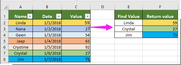
다음 스크린샷과 같은 테이블이 있다고 가정합니다. 이제 열 A 에 특정 값이 있는지 확인한 후 해당 값과 함께 열 C 의 배경색을(를) 반환하려고 합니다。 이를 어떻게 구현할 수 있을까요? 이 문서에서 소개하는 방법이 문제 해결에 도움이 될 수 있습니다。
사용자 정의 함수를 사용하여 VLOOKUP 하고 조회 값과 함께 배경색을(를) 반환하기
사용자 정의 함수를 사용하여 VLOOKUP 하고 조회 값과 함께 배경색을(를) 반환하기
Excel 에서 값을 조회하고 해당 값과 함께 배경색을(를) 반환하려면 다음 단계를 따르세요。
1. VLOOKUP 하려는 값을 포함한 워크시트에서 시트 탭을 마우스 오른쪽 버튼으로 클릭하고코드 보기을(를) 상황에 맞는 메뉴에서 선택하세요。 스크린샷 참조:

2. 열리는Microsoft Visual Basic for Applications창에서 아래 VBA 코드를 코드 창에 복사하세요。
VBA 코드 1: VLOOKUP 하고 조회 값과 함께 배경색을(를) 반환하기
Sub Worksheet_Change(ByVal Target As Range)
    Dim I As Long
    Dim xKeys As Long
    Dim xDicStr As String
    On Error Resume Next
    Application.ScreenUpdating = False
    xKeys = UBound(xDic.Keys)
    If xKeys >= 0 Then
        For I = 0 To UBound(xDic.Keys)
            xDicStr = xDic.Items(I)
            If xDicStr <> "" Then
                Range(xDic.Keys(I)).Interior.Color = _
                Range(xDic.Items(I)).Interior.Color
            Else
                Range(xDic.Keys(I)).Interior.Color = xlNone
            End If
        Next
        Set xDic = Nothing
    End If
    Application.ScreenUpdating = True
End Sub
3. 그런 다음삽입>모듈을 클릭하고 아래 VBA 코드 2 을 모듈 창에 복사하세요。
VBA 코드 2: VLOOKUP 하고 조회 값과 함께 배경색을(를) 반환하기
Public xDic As New Dictionary
Function LookupKeepColor (ByRef FndValue, ByRef LookupRng As Range, ByRef xCol As Long)
    Dim xFindCell As Range
    On Error Resume Next
    Set xFindCell = LookupRng.Find(FndValue, , xlValues, xlWhole)
    If xFindCell Is Nothing Then
        LookupKeepColor = ""
        xDic.Add Application.Caller.Address, ""
    Else
        LookupKeepColor = xFindCell.Offset(0, xCol - 1).Value
        xDic.Add Application.Caller.Address, xFindCell.Offset(0, xCol - 1).Address
    End If
End Function
4. 두 코드를 삽입한 후도구>참조을 클릭하세요。 그런 다음Microsoft Script Runtime상자를참조 – VBAProject대화 상자에서 선택하세요。 스크린샷 참조:

5. Alt+Q키를 눌러Microsoft Visual Basic for Applications창을 닫고 워크시트로 돌아가세요。
6. 조회 값 옆의 빈 셀을 선택한 후 수식=LookupKeepColor(E2,$A$1:$C$8,3)을(를) 수식 표시줄에 입력하고 Enter 키를 누르세요。

참고: 수식에서E2는 조회할 값을 포함하고,$A$1:$C$8는 테이블 범위이며, 숫자3은 반환할 해당 값이 테이블의 세 번째 열에 있음을 의미합니다。 필요에 따라 값을 변경하세요。
7. 첫 번째 결과 셀을 계속 선택한 상태에서 채우기 핸들을 아래로 드래그하여 모든 결과와 해당 배경색을(를) 가져오세요。 스크린샷 참조。

관련 문서:
- Excel 에서 VLOOKUP 을 사용할 때 조회 셀의 원본 서식을 복사하려면 어떻게 하나요?
- Excel 에서 VLOOKUP 을 수행하고 숫자 대신 날짜 형식을(를) 반환하려면 어떻게 하나요?
- Excel 에서 VLOOKUP 과 SUM 을 함께 사용하려면 어떻게 하나요?
- Excel 에서 인접하거나 다음 셀에서 반환 값을(를) VLOOKUP 하려면 어떻게 하나요?
- Excel 에서 VLOOKUP 값을 조회하여 TRUE 또는 FALSE / YES 또는 NO 로 반환하려면 어떻게 하나요?
최고의 Office 생산성 도구
| 🤖 | KUTOOLS AI 도우미: 다음을 기반으로 데이터 분석 혁신하기:지능형 실행 | 코드 생성| 사용자 지정 수식 생성 | 데이터 분석 및 차트 생성| 향상된 함수 호출… |
| 인기 기능:찾기, 강조 표시 또는 중복 표시 | 빈 행 삭제 | 데이터 손실 없이 열 결합 또는 셀 제거 | 공식을 사용하지 않는 반올림... | |
| 슈퍼 LOOKUP:다중 조건 VLookup | 다중 값 VLookup | 여러 시트에서 VLookup | 퍼지 매치.... | |
| 고급 드롭다운 목록:드롭다운 목록 빠르게 생성 | 종속형 드롭다운 목록 | 다중 선택 드롭다운 목록.... | |
| 열 관리자:특정 수의 열 추가|열 이동|숨겨진 열의 표시 상태 전환|범위 및 열 비교... | |
| 주요 기능:그리드 포커스 | 디자인 보기 |향상된 수식 표시줄 | 워크북 및 시트 관리자 | 자원 라이브러리(자동 텍스트)| 날짜 선택기 | 워크시트 병합 | 암호화/셀 해독 | 목록으로 이메일 보내기 | 슈퍼 필터 | 특수 필터(굵은 글꼴이 있는 셀 필터링/기울임꼴/취소선。。。) 。。。 | |
| 상위 15 도구 모음:12 텍스트도구(텍스트 추가,특정 문자 삭제, ...)| 50+차트유형(간트 차트, ...)| 40+ 실용적인수식(생일을 기준으로 나이 계산, ...)| 19 삽입도구(QR 코드 삽입,경로에서 그림 삽입, ...)| 12 변환도구(단어로 변환하기,환율 변환, ...)| 7 병합 및 분할도구(고급 행 병합,셀 분할, ...)|그 외 더 많은 기능 |
Kutools for Excel 로 Excel 역량을 한 단계 업그레이드하고 전례 없는 효율성을 경험하세요。Kutools for Excel 는 생산성과 저장 시간을 향상시키는 300 개 이상의 고급 기능을 제공합니다。가장 필요한 기능을 지금 바로 확인하세요。。。
Office Tab 가 Office 에 탭 인터페이스를 제공하여 작업을 훨씬 쉽게 만들어 줍니다
- Word, Excel, PowerPoint 에서 탭 기반 편집 및 읽기 기능을 활성화합니다, Publisher, Access, Visio 및 Project 에서도 사용 가능합니다。
- 새 창이 아닌 동일한 창의 새 탭에서 여러 문서를 열고 생성할 수 있습니다。
- 50% 만큼 생산성을 높이고 매일 수백 번의 마우스 클릭을 줄여줍니다!
모든 Kutools 애드인。 하나의 설치 프로그램
Kutools for Office스위트 번들은 Excel, Word, Outlook 및 PowerPoint 용 애드인과 Office Tab Pro 를 포함하며, 다양한 Office 앱을 사용하는 팀에 이상적입니다。
- 올인원 스위트— Excel, Word, Outlook 및 PowerPoint 애드인 + Office Tab Pro
- 하나의 설치 프로그램, 하나의 라이선스— 몇 분 안에 설정 완료(MSI 지원)
- 함께 사용할수록 더 효과적입니다— Office 앱 전반에서 생산성 향상
- 30 일간 모든 기능 무료 체험— 등록이나 신용카드 필요 없음
- 최고의 가성비— 개별 애드인 구매 대비 절약