Google 시트에서 다른 시트를 기반으로 조건부 서식을 적용하는 방법은 무엇입니까?
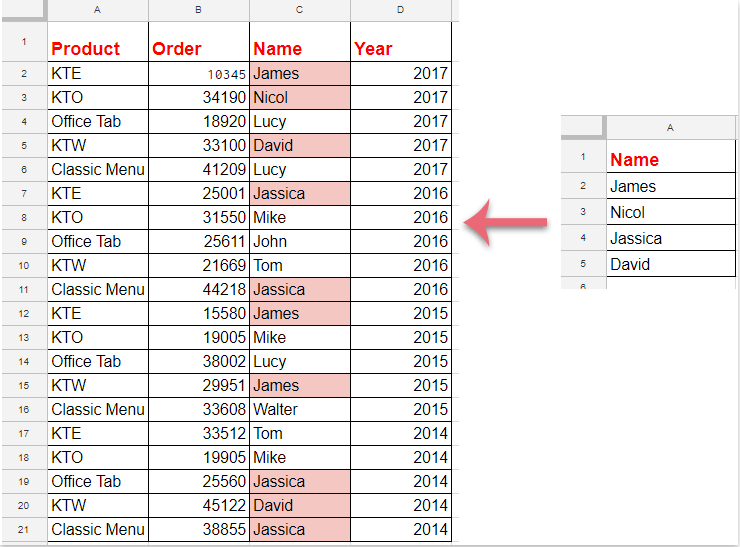
조건부 서식은 Google 시트에서 특정 기준에 따라 셀을 자동으로 강조 표시할 수 있는 유용한 기능으로, 데이터를 분석하고 시각화하기 쉽게 만듭니다. 때로는 동일한 시트 내의 값에 따라 셀을 강조 표시하는 대신, 다른 시트에 저장된 참조 목록이나 기준에 따라 서식 규칙을 설정해야 할 수도 있습니다. 예를 들어, 아래 스크린샷에서 보여지는 것처럼 한 시트에서 다른 시트에 유지 관리되는 목록에 나타나는 셀을 강조 표시하려고 할 수 있습니다. 이와 같은 작업은 현재 판매량을 마스터 제품 목록과 비교하거나 다른 데이터 소스에 대해 중복 항목을 확인하는 등, 상호 참조 데이터를 다룰 때 흔히 발생합니다. 하지만 특히 여러 시트 간 데이터를 참조할 때 Google 시트에서 이러한 조건부 서식을 설정하는 것은 이전에 해본 적이 없다면 혼란스러울 수 있습니다. 아래 가이드에서는 이를 단계별로 쉽게 해결하는 방법을 안내합니다.
Google 시트에서 다른 시트의 목록을 기반으로 조건부 서식을 적용하여 셀 강조하기
Google 시트에서 다른 시트의 목록을 기반으로 조건부 서식을 적용하여 셀 강조하기
이 방법은 활성 시트에서 지정된 다른 시트의 목록에 포함된 경우 셀을 강조 표시하는 조건부 서식 규칙을 설정할 수 있게 해줍니다. 특히 동적 데이터 모니터링 및 관련 데이터 세트 간 일관성 유지에 있어서 이러한 시트 간 조건부 서식은 매우 유용합니다.
이 과정을 완료하려면 다음의 상세 단계를 따르세요:
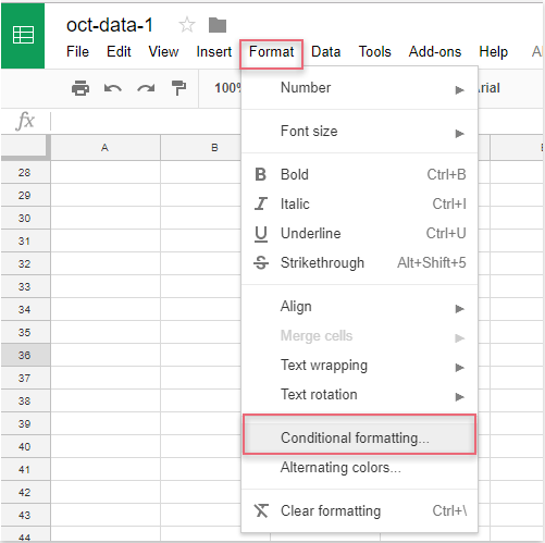
1. 대상 워크시트를 열고 상단의 서식 메뉴를 클릭한 후 조건부 서식을 선택하세요. 그러면 화면 오른쪽에 조건부 서식 규칙 창이 열립니다.
2. 조건부 서식 규칙 패널에서 다음 작업을 수행하세요:
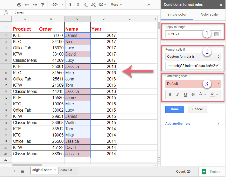
(1.) "적용 범위" 필드 옆의 ![]() 버튼을 클릭하세요. 서식을 적용하고자 하는 셀 범위를 선택하세요. 예를 들어, C열의 2행부터 모든 값을 서식화하려면 C2:C를 선택하세요. 적절한 범위를 선택하면 의도한 셀만 서식 평가 대상이 됩니다.
버튼을 클릭하세요. 서식을 적용하고자 하는 셀 범위를 선택하세요. 예를 들어, C열의 2행부터 모든 값을 서식화하려면 C2:C를 선택하세요. 적절한 범위를 선택하면 의도한 셀만 서식 평가 대상이 됩니다.
(2.) 셀 서식 지정 조건 드롭다운 메뉴에서 '사용자 정의 수식 사용'을 선택하세요. 그리고 제공된 박스에 다음 수식을 입력하세요: =match(C2,indirect("data list!A2:A"),0). 이 수식은 C열의 각 셀이 'data list' 시트의 A2:A 범위에 포함되는지 여부를 확인합니다.
(3.) 서식 스타일 섹션에서 원하는 서식을 선택하세요. 예를 들어 특정 색상으로 셀을 채우거나 글꼴 스타일을 변경할 수 있습니다. 서식을 적용하기 전에 바로 시트에서 스타일을 미리 볼 수 있습니다.
참고: 위 수식에서 C2는 선택된 범위의 첫 번째 셀을 의미합니다 (데이터가 다른 행이나 열에서 시작하는 경우 조정 필요). data list!A2:A는 다른 시트에 저장된 목록을 가리키며, 여기서 'data list'는 시트 이름이고 A2:A는 해당 범위입니다. 수식에서 셀 참조가 선택된 범위의 좌측 상단 셀과 일치하는지 확인하세요. 그렇지 않으면 서식이 제대로 적용되지 않을 수 있습니다. 데이터 목록 범위가 다른 경우 수식에서도 업데이트해야 합니다 (예: “data list!B2:B”).
3. 규칙을 설정한 후 선택된 범위 내에서 매칭되는 셀은 즉시 다른 시트의 목록에 기반하여 강조 표시됩니다. 미리보기를 검토한 후 조건부 서식 규칙 창 하단의 완료 버튼을 클릭하여 서식을 적용하고 저장하세요.
팁 및 문제 해결:
- 수식에서 오타를 다시 확인하세요. 특히 시트 이름과 범위 참조에 주의하세요—잘못된 참조는 규칙이 적용되지 않는 일반적인 이유입니다.
- 데이터 목록에 빈 셀이 포함된 경우,
MATCH함수는 매칭되지 않는 값에 대해#N/A오류를 반환하지만, 이는 예상되는 동작이며 매칭되는 항목의 강조에는 영향을 미치지 않습니다. - 새로운 시트로 서식을 복사하거나 범위를 조정할 때 사용자 정의 수식의 셀 참조도 그에 맞게 업데이트해야 합니다.
- 참조 목록에 나중에 항목을 추가하거나 삭제하면 서식이 자동으로 업데이트됩니다.
- 수식에서 참조하는 시트와 범위가 존재하며, 올바르게 표기되어 있는지 확인하세요.
- 수식의 첫 번째 셀이 선택된 범위의 첫 번째 셀과 일치하는지 확인하세요.
- 스프레드시트 내에서 시트 간 접근에 필요한 모든 권한이 부여되었는지 확인하세요—이 방법은 단일 멀티 시트 Google 시트 파일 내에서 작동하며, 다른 파일 간에는 작동하지 않습니다.
대안적으로, 데이터 구조 또는 요구사항이 더 복잡한 경우 (예: 여러 열을 비교하거나 부분 일치를 허용하거나 고급 조회를 수행해야 하는 경우) COUNTIF 또는 VLOOKUP 수식을 활용한 도우미 열을 사용하거나 Google Apps Script (사용자 정의 JavaScript 코드)를 사용하여 유연한 조건부 서식 솔루션을 구현할 수도 있습니다.
요약하자면, 다른 시트를 기반으로 조건부 서식을 설정하는 것은 목록 확인, 중복 추적 및 다양한 시트 간 데이터 검증에 매우 효과적입니다—모두 Google 시트 내에서 가능합니다. 항상 수식 입력값, 참조 범위 및 서식 규칙을 확인하여 원활하고 정확한 결과를 얻으세요.

Kutools AI로 엑셀의 마법을 풀다
- 스마트 실행: 셀 작업 수행, 데이터 분석 및 차트 생성 - 간단한 명령어로 모든 것을 처리합니다.
- 사용자 정의 수식: 작업을 간소화하기 위한 맞춤형 수식을 생성합니다.
- VBA 코딩: 손쉽게 VBA 코드를 작성하고 실행합니다.
- 수식 해석: 복잡한 수식도 쉽게 이해할 수 있습니다.
- 텍스트 번역: 스프레드시트 내 언어 장벽을 허물어 보세요.
최고의 오피스 생산성 도구
| 🤖 | Kutools AI 도우미: 데이터 분석에 혁신을 가져옵니다. 방법: 지능형 실행 | 코드 생성 | 사용자 정의 수식 생성 | 데이터 분석 및 차트 생성 | Kutools Functions 호출… |
| 인기 기능: 중복 찾기, 강조 또는 중복 표시 | 빈 행 삭제 | 데이터 손실 없이 열 또는 셀 병합 | 반올림(수식 없이) ... | |
| 슈퍼 LOOKUP: 다중 조건 VLOOKUP | 다중 값 VLOOKUP | 다중 시트 조회 | 퍼지 매치 .... | |
| 고급 드롭다운 목록: 드롭다운 목록 빠르게 생성 | 종속 드롭다운 목록 | 다중 선택 드롭다운 목록 .... | |
| 열 관리자: 지정한 수의 열 추가 | 열 이동 | 숨겨진 열의 표시 상태 전환 | 범위 및 열 비교 ... | |
| 추천 기능: 그리드 포커스 | 디자인 보기 | 향상된 수식 표시줄 | 통합 문서 & 시트 관리자 | 자동 텍스트 라이브러리 | 날짜 선택기 | 데이터 병합 | 셀 암호화/해독 | 목록으로 이메일 보내기 | 슈퍼 필터 | 특수 필터(굵게/이탤릭/취소선 필터 등) ... | |
| 15대 주요 도구 세트: 12 가지 텍스트 도구(텍스트 추가, 특정 문자 삭제, ...) | 50+ 종류의 차트(간트 차트, ...) | 40+ 실용적 수식(생일을 기반으로 나이 계산, ...) | 19 가지 삽입 도구(QR 코드 삽입, 경로에서 그림 삽입, ...) | 12 가지 변환 도구(단어로 변환하기, 통화 변환, ...) | 7 가지 병합 & 분할 도구(고급 행 병합, 셀 분할, ...) | ... 등 다양 |
Kutools for Excel과 함께 엑셀 능력을 한 단계 끌어 올리고, 이전에 없던 효율성을 경험하세요. Kutools for Excel은300개 이상의 고급 기능으로 생산성을 높이고 저장 시간을 단축합니다. 가장 필요한 기능을 바로 확인하려면 여기를 클릭하세요...
Office Tab은 Office에 탭 인터페이스를 제공하여 작업을 더욱 간편하게 만듭니다
- Word, Excel, PowerPoint에서 탭 편집 및 읽기를 활성화합니다.
- 새 창 대신 같은 창의 새로운 탭에서 여러 파일을 열고 생성할 수 있습니다.
- 생산성이50% 증가하며, 매일 수백 번의 마우스 클릭을 줄여줍니다!
모든 Kutools 추가 기능. 한 번에 설치
Kutools for Office 제품군은 Excel, Word, Outlook, PowerPoint용 추가 기능과 Office Tab Pro를 한 번에 제공하여 Office 앱을 활용하는 팀에 최적입니다.
- 올인원 제품군 — Excel, Word, Outlook, PowerPoint 추가 기능 + Office Tab Pro
- 설치 한 번, 라이선스 한 번 — 몇 분 만에 손쉽게 설정(MSI 지원)
- 함께 사용할 때 더욱 효율적 — Office 앱 간 생산성 향상
- 30일 모든 기능 사용 가능 — 회원가입/카드 불필요
- 최고의 가성비 — 개별 추가 기능 구매 대비 절약