체크박스로 Excel에서 셀 또는 행 강조하는 방법은 무엇입니까?
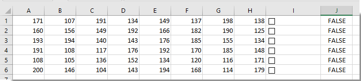
아래 스크린샷에 표시된 대로 체크박스로 행이나 셀을 강조해야 합니다. 체크박스가 선택되면 지정된 행이나 셀이 자동으로 강조됩니다. 하지만 Excel에서 이를 어떻게 구현할 수 있을까요? 이 문서에서는 이를 달성하기 위한 두 가지 방법을 보여드리겠습니다.

조건부 서식을 사용하여 체크박스로 셀 또는 행 강조
VBA 코드를 사용하여 체크박스로 셀 또는 행 강조
조건부 서식을 사용하여 체크박스로 셀 또는 행 강조
Excel에서 체크박스로 셀 또는 행을 강조하기 위해 조건부 서식 규칙을 생성할 수 있습니다. 아래 단계를 따라 주세요.
첫 번째 단계: 모든 체크박스를 특정 셀에 연결
1. 개발 도구 > 삽입 > 체크박스 (양식 컨트롤)을 클릭하여 하나씩 수동으로 셀에 체크박스를 삽입해야 합니다.
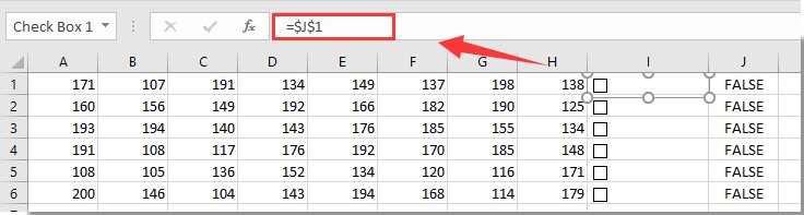
2. 이제 체크박스가 I열의 셀에 삽입되었습니다. I1의 첫 번째 체크박스를 선택하고, 수식 표시줄에 =$J1 공식을 입력한 다음 Enter 키를 누릅니다.
팁: 체크박스와 인접한 셀에 값이 연관되지 않기를 원한다면, 다른 워크시트의 셀에 체크박스를 연결할 수 있습니다. 예: =Sheet3!$E1.
3. 모든 체크박스가 인접한 셀이나 다른 워크시트의 셀에 연결될 때까지 1단계를 반복합니다.
참고: 모든 연결된 셀은 연속적이어야 하며 동일한 열에 있어야 합니다.
두 번째 단계: 조건부 서식 규칙 생성
이제 다음과 같은 단계를 통해 조건부 서식 규칙을 생성해야 합니다.
1. 체크박스로 강조해야 할 행을 선택한 다음 홈 탭에서 조건부 서식 > 새 규칙을 클릭합니다. 스크린샷 참조:

2. 새 서식 규칙 대화 상자에서 다음을 수행해야 합니다:
2.1 규칙 유형 선택 박스에서 수식을 사용하여 서식을 지정할 셀을 결정 옵션을 선택합니다;
2.2 공식 입력 =IF($J1=TRUE,TRUE,FALSE) 다음과 같이 이 공식이 참인 경우 값을 서식 지정 상자에;
혹은 =IF(Sheet3!$E1=TRUE,TRUE,FALSE) 체크박스가 다른 워크시트에 연결된 경우.
2.3 서식 버튼을 클릭하여 행에 대한 강조 색상을 지정합니다;
2.4 확인 버튼을 클릭합니다. 스크린샷 참조:

참고: 공식에서 $J1 또는 $E1은 체크박스의 첫 번째 연결된 셀이며, 셀 참조가 열 절대값(J1 > $J1 또는 E1 > $E1)으로 변경되었는지 확인하십시오.
이제 조건부 서식 규칙이 생성되었습니다. 체크박스를 선택하면 해당 행이 아래 스크린샷에 표시된 대로 자동으로 강조됩니다.

VBA 코드를 사용하여 체크박스로 셀 또는 행 강조
다음 VBA 코드는 또한 Excel에서 체크박스로 셀 또는 행을 강조하는 데 도움이 될 수 있습니다. 아래 단계를 따라 주세요.
1. 체크박스로 셀 또는 행을 강조해야 하는 워크시트에서 시트 탭을 마우스 오른쪽 버튼으로 클릭하고 바로 가기 메뉴에서 코드 보기(V)를 선택하여 Microsoft Visual Basic for Applications 창을 엽니다.
2. 그런 다음 아래 VBA 코드를 코드 창에 복사하여 붙여넣습니다.
VBA 코드: Excel에서 체크박스로 행 강조
Sub AddCheckBox()
Dim xCell As Range
Dim xRng As Range
Dim I As Integer
Dim xChk As CheckBox
On Error Resume Next
InputC:
    Set xRng = Application.InputBox("Please select the column range to insert checkboxes:", "Kutools for Excel", Selection.Address, , , , , 8)
If xRng Is Nothing Then Exit Sub
If xRng.Columns.Count > 1 Then
    MsgBox "The selected range should be a single column", vbInformation, "Kutools fro Excel"
    GoTo InputC
Else
    If xRng.Columns.Count = 1 Then
        For Each xCell In xRng
            With ActiveSheet.CheckBoxes.Add(xCell.Left, _
               xCell.Top, xCell.Width = 15, xCell.Height = 12)
               .LinkedCell = xCell.Offset(, 1).Address(External:=False)
               .Interior.ColorIndex = xlNone
               .Caption = ""
               .Name = "Check Box " & xCell.Row
            End With
            xRng.Rows(xCell.Row).Interior.ColorIndex = xlNone
        Next
    End If
    With xRng
     .Rows.RowHeight = 16
    End With
    xRng.ColumnWidth = 5#
    xRng.Cells(1, 1).Offset(0, 1).Select
    For Each xChk In ActiveSheet.CheckBoxes
      xChk.OnAction = ActiveSheet.Name + ".InsertBgColor"
    Next
End If
End Sub

Sub InsertBgColor()
Dim xName As Integer
Dim xChk As CheckBox
For Each xChk In ActiveSheet.CheckBoxes
  xName = Right(xChk.Name, Len(xChk.Name) - 10)
  If (xName = Range(xChk.LinkedCell).Row) Then
   If (Range(xChk.LinkedCell) = "True") Then
    Range("A" & xName, Range(xChk.LinkedCell).Offset(0, -2)).Interior.ColorIndex = 6
   Else
    Range("A" & xName, Range(xChk.LinkedCell).Offset(0, -2)).Interior.ColorIndex = xlNone
   End If
  End If
Next
End Sub
3. F5 키를 눌러 코드를 실행합니다. (참고: F5 키를 적용하려면 커서를 코드의 첫 부분에 놓아야 함). 팝업되는 Kutools for Excel 대화 상자에서 체크박스를 삽입하려는 범위를 선택한 다음 확인 버튼을 클릭합니다. 여기서는 I1:I6 범위를 선택했습니다. 스크린샷 참조:

4. 그런 다음 체크박스가 선택된 셀에 삽입됩니다. 체크박스 중 하나를 선택하면 해당 행이 아래 스크린샷에 표시된 대로 자동으로 강조됩니다.

관련 기사:
- Excel에서 체크박스가 선택되었을 때 특정 셀 값 또는 색상을 변경하는 방법은 무엇입니까?
- Excel에서 체크박스를 선택했을 때 셀에 날짜 스탬프를 삽입하는 방법은 무엇입니까?
- Excel에서 셀 값에 따라 체크박스를 선택하는 방법은 무엇입니까?
- Excel에서 체크박스를 기반으로 데이터를 필터링하는 방법은 무엇입니까?
- Excel에서 행이 숨겨졌을 때 체크박스를 숨기는 방법은 무엇입니까?
- Excel에서 여러 체크박스가 있는 드롭다운 목록을 만드는 방법은 무엇입니까?
최고의 오피스 생산성 도구
| 🤖 | Kutools AI 도우미: 데이터 분석에 혁신을 가져옵니다. 방법: 지능형 실행 | 코드 생성 | 사용자 정의 수식 생성 | 데이터 분석 및 차트 생성 | Kutools Functions 호출… |
| 인기 기능: 중복 찾기, 강조 또는 중복 표시 | 빈 행 삭제 | 데이터 손실 없이 열 또는 셀 병합 | 반올림(수식 없이) ... | |
| 슈퍼 LOOKUP: 다중 조건 VLOOKUP | 다중 값 VLOOKUP | 다중 시트 조회 | 퍼지 매치 .... | |
| 고급 드롭다운 목록: 드롭다운 목록 빠르게 생성 | 종속 드롭다운 목록 | 다중 선택 드롭다운 목록 .... | |
| 열 관리자: 지정한 수의 열 추가 | 열 이동 | 숨겨진 열의 표시 상태 전환 | 범위 및 열 비교 ... | |
| 추천 기능: 그리드 포커스 | 디자인 보기 | 향상된 수식 표시줄 | 통합 문서 & 시트 관리자 | 자동 텍스트 라이브러리 | 날짜 선택기 | 데이터 병합 | 셀 암호화/해독 | 목록으로 이메일 보내기 | 슈퍼 필터 | 특수 필터(굵게/이탤릭/취소선 필터 등) ... | |
| 15대 주요 도구 세트: 12 가지 텍스트 도구(텍스트 추가, 특정 문자 삭제, ...) | 50+ 종류의 차트(간트 차트, ...) | 40+ 실용적 수식(생일을 기반으로 나이 계산, ...) | 19 가지 삽입 도구(QR 코드 삽입, 경로에서 그림 삽입, ...) | 12 가지 변환 도구(단어로 변환하기, 통화 변환, ...) | 7 가지 병합 & 분할 도구(고급 행 병합, 셀 분할, ...) | ... 등 다양 |
Kutools for Excel과 함께 엑셀 능력을 한 단계 끌어 올리고, 이전에 없던 효율성을 경험하세요. Kutools for Excel은300개 이상의 고급 기능으로 생산성을 높이고 저장 시간을 단축합니다. 가장 필요한 기능을 바로 확인하려면 여기를 클릭하세요...
Office Tab은 Office에 탭 인터페이스를 제공하여 작업을 더욱 간편하게 만듭니다
- Word, Excel, PowerPoint에서 탭 편집 및 읽기를 활성화합니다.
- 새 창 대신 같은 창의 새로운 탭에서 여러 파일을 열고 생성할 수 있습니다.
- 생산성이50% 증가하며, 매일 수백 번의 마우스 클릭을 줄여줍니다!
모든 Kutools 추가 기능. 한 번에 설치
Kutools for Office 제품군은 Excel, Word, Outlook, PowerPoint용 추가 기능과 Office Tab Pro를 한 번에 제공하여 Office 앱을 활용하는 팀에 최적입니다.
- 올인원 제품군 — Excel, Word, Outlook, PowerPoint 추가 기능 + Office Tab Pro
- 설치 한 번, 라이선스 한 번 — 몇 분 만에 손쉽게 설정(MSI 지원)
- 함께 사용할 때 더욱 효율적 — Office 앱 간 생산성 향상
- 30일 모든 기능 사용 가능 — 회원가입/카드 불필요
- 최고의 가성비 — 개별 추가 기능 구매 대비 절약