Excel 에서 VLOOKUP 으로 여러 개의 대응 값을 조회하고 연결하려면 어떻게 해야 하나요？

Excel 에서 VLOOKUP 함수는 일반적으로 주어진 조회 기준에 대해 처음 발견된 일치 값을 반환합니다。 그러나 특정 키와 관련된 모든 일치 값을 검색하고 결합해야 하는 경우가 많습니다。 예를 들어 한 반의 모든 학생 목록을 만들거나 특정 카테고리에 속한 모든 제품을 나열해야 할 때 그렇습니다。 표준 VLOOKUP 함수는 이러한 요구사항을 충족시키지 못하므로， 단일 셀에 여러 개의 대응 결과를 동시에 조회하고 연결하는 방법을 고민하게 됩니다。 아래에서는 Excel 버전과 사용자 선호도에 따라 활용할 수 있는 몇 가지 실용적이고 효율적인 방법을 소개합니다。

Excel 에서 VLOOKUP 으로 여러 개의 대응 값을 조회하고 연결하기

• TEXTJOIN 및 FILTER 함수 사용하기(Excel 365/2021)
• Kutools for Excel 사용하기
• 사용자 정의 함수 사용하기
• 다중 연결을 위한 VBA 코드 사용하기

TEXTJOIN 및 FILTER 함수로 VLOOKUP 과 여러 개의 대응 값을 연결하기

Excel 365 또는 Excel 2021 를 사용 중이라면 TEXTJOIN 과 FILTER 함수를 조합하여 효율적으로 수식 기반의 해결책을 적용할 수 있습니다。 이 방법은 특히 동적이고 자주 업데이트되는 데이터셋에 적합하며， 원본 데이터이 변경되면 결과가 자동으로 새로 고쳐집니다。 FILTER 함수를 지원하는 최신 Office 버전에서만 사용 가능하므로， 해당 기능을 사용하기 전 Excel 버전을 확인하는 것이 좋습니다。

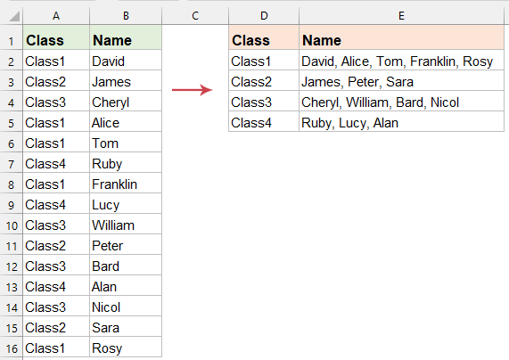
대상 셀에 다음 수식을 입력한 후， 다른 행에도 적용하려면 수식을 아래로 드래그합니다。 모든 대응되는 일치 값이 추출되어 하나의 셀에 연결됩니다。 스크린샷 참조：

=TEXTJOIN(", ", TRUE, FILTER($B$2:$B$16, $A$2:$A$16=D2, ""))

Kutools for Excel 로 VLOOKUP 과 여러 개의 대응 값을 연결하기

내장 수식 방법이 복잡하게 느껴지거나 TEXTJOIN 및 FILTER 와 같은 고급 함수를 지원하지 않는 Excel 버전을 사용 중이라면, Kutools for Excel 이 직관적인 그래픽 인터페이스를 제공합니다. Kutools 의 일대다 조회 기능을 사용하면 몇 번의 클릭만으로 여러 개의 일치 결과를 조회하고 연결할 수 있어 초보자부터 고급 사용자까지 모두에게 적합합니다. Kutools 를 사용하면 복잡한 수식이나 코드를 작성할 필요가 없으며， 반복적인 조회 및 집계가 필요한 대규모 또는 가변적인 데이터셋을 다룰 때 특히 유용합니다。

Kutools for Excel 설치 후 다음 단계를 따르세요：

클릭Kutools>슈퍼 LOOKUP>일대다 조회(여러 결과 반환)하여 설정 대화 상자를 엽니다。 이 대화 상자 내에서 다음 단계에 따라 조회 및 출력 설정을 빠르게 구성할 수 있습니다：

1. 연결 결과를 표시할 대상 셀과 검색하고자 하는 값을 포함한 셀을 선택합니다。
2. 조회 키와 결과 열을 모두 포함하는 테이블 범위를 지정합니다。
3. 조회 키가 포함된 열(키 열)과 연결할 값을 포함한 열(반환 열)을 각각 지정합니다。
4. 확인 버튼을 클릭하여 설정을 완료하고 데이터를 처리합니다。
   

결과: Kutools 가 선택한 출력 셀에 모든 일치 값과 연결 결과를 표시합니다。 스크린샷 참조：

이 방법은 복잡한 수식이나 코드 없이 Excel 인터페이스에서 작업하려는 사용자에게 강력히 권장됩니다。 또한 수식 오류 가능성을 줄이고 반복적인 조회 및 연결 작업의 생산성을 높여줍니다。

사용자 정의 함수로 VLOOKUP 과 여러 개의 대응 값을 연결하기

VBA(Visual Basic for Applications)에 능숙하거나 FILTER 함수와 같은 동적 배열 기능을 지원하지 않는 이전 Excel 버전을 사용 중인 경우， 맞춤형 사용자 정의 함수(UDF)를 만들어 여러 결과를 유연하게 연결할 수 있습니다。 이 방법은 모든 Excel 버전과 호환되며， 특정 구분자나 조건에 맞게 조정할 수 있습니다。

1. ALT + F11키를 누른 상태로 유지하여Microsoft Visual Basic for Applications창을 엽니다。

2. 클릭삽입>모듈， 그런 다음 다음 코드를 모듈 창에 붙여넣습니다。

VBA 코드: 셀 내에서 VLOOKUP 으로 여러 개의 일치 값을 조회하고 연결하기

Function ConcatenateMatches(LookupValue As String, LookupRange As Range, ReturnRange As Range, Optional Delimiter As String = ", ") As String
'Updateby Extendoffice
    Dim Cell As Range
    Dim Result As String
    Result = ""
    For Each Cell In LookupRange
        If Cell.Value = LookupValue Then
            Result = Result & Cell.Offset(0, ReturnRange.Column - LookupRange.Column).Value & Delimiter
        End If
    Next Cell
    If Result <> "" Then
        Result = Left(Result, Len(Result) - Len(Delimiter))
    End If
    ConcatenateMatches = Result
End Function

3. VBA 편집기를 저장하고 닫기합니다. 워크시트로 돌아가서 결과를 표시할 빈 셀에 다음 수식을 입력하여 이 UDF 를 사용합니다：=ConcatenateMatches(D2, $A$2:$A$16, $B$2:$B$16)。 필요에 따라 채우기 핸들을 아래로 드래그하여 다른 셀에도 수식을 복사합니다。 특정 조회 값에 기반한 모든 대응 값이 콤마와 공백으로 구분되어 하나의 셀에 반환되고 연결됩니다。 스크린샷 참조：

VBA 코드로 VLOOKUP 과 여러 개의 대응 값을 연결하기

반복적으로 사용해야 하거나 워크시트 셀에 사용자 정의 함수를 삽입하지 않으려는 경우， 미리 준비된 VBA 매크로를 사용하여 결과를 직접 연결할 수 있습니다。 이 방법은 모든 사용자가 동일한 Excel 버전이나 애드인을 보유하지 않은 공유 환경에서도 잘 작동합니다。

1. 클릭개발자 도구>Visual Basic하여 VBA 편집기를 엽니다。

2. VBA 창에서 클릭삽입>모듈， 그런 다음 다음 코드를 모듈에 붙여넣습니다：

Sub VLookupAndConcatenate()
    Dim ws As Worksheet
    Dim dataRange As Range, lookupRange As Range, resultRange As Range
    Dim dict As Object
    Dim i As Long, lastRow As Long
    Dim lookupValue As Variant, result As String
    Dim delimiter As String
    delimiter = ", "
    Set dict = CreateObject("Scripting.Dictionary")
    Set ws = ActiveSheet
    On Error Resume Next
    Set dataRange = Application.InputBox( _
        Prompt:="Please select the data range (contains lookup column and result column)", _
        Title:="Select Data Range", _
        Type:=8)
    On Error GoTo 0
    If dataRange Is Nothing Then Exit Sub
    On Error Resume Next
    Set lookupRange = Application.InputBox( _
        Prompt:="Please select the lookup range (single column)", _
        Title:="Select Lookup Range", _
        Type:=8)
    On Error GoTo 0
    If lookupRange Is Nothing Then Exit Sub
    On Error Resume Next
    Set resultRange = Application.InputBox( _
        Prompt:="Please select the starting cell for results output", _
        Title:="Select Output Location", _
        Type:=8)
    On Error GoTo 0
    If resultRange Is Nothing Then Exit Sub
    resultRange.Resize(lookupRange.Rows.Count, 1).ClearContents
    For i = 1 To dataRange.Rows.Count
        lookupValue = dataRange.Cells(i, 1).Value
        If Not dict.Exists(lookupValue) Then
            dict.Add lookupValue, dataRange.Cells(i, 2).Value
        Else
            dict(lookupValue) = dict(lookupValue) & delimiter & dataRange.Cells(i, 2).Value
        End If
    Next i
    For i = 1 To lookupRange.Rows.Count
        lookupValue = lookupRange.Cells(i, 1).Value
        If dict.Exists(lookupValue) Then
            resultRange.Cells(i, 1).Value = dict(lookupValue)
        Else
            resultRange.Cells(i, 1).Value = "Not Found"
        End If
    Next i
    MsgBox "Operation completed! Processed " & lookupRange.Rows.Count & " lookup values.", vbInformation
End Sub

3. 실행 버튼을 클릭하여 매크로를 실행합니다。 입력 상자가 나타나 데이터 범위， 조회 범위， 결과 범위를 선택하라는 메시지를 표시합니다。 연결된 결과는 선택한 출력 셀에 바로 표시됩니다。

이 매크로 방식은 다른 값로 여러 번 연결 검색을 수행해야 하는 경우 특히 유용하며， 워크시트에 UDF 호출이 난잡하게 퍼지는 것을 방지합니다。

필요 시 코드 내 구분자를 쉽게 조정할 수 있으며， 워크플로에 따라 결과를 셀이나 파일로 출력하도록 매크로를 확장할 수도 있습니다。

Excel 에서 여러 개의 대응하는 값을 연결하는 작업은 다양한 방법으로 가능하며, 각 방법은 상황에 따라 특정한 장점을 제공합니다. 동적 배열 수식, Kutools for Excel 과 같은 애드인， 또는 VBA 기반 방법 중 어느 것을 선택하든 그룹화된 데이터를 효율적으로 분석하고 표시하는 능력이 향상됩니다。 데이터셋의 크기와 복잡도에 따라 성능과 유지보수 측면에서 자신이나 팀에 가장 적합한 방법을 고려해 보세요。 일상적인 작업에서는 데이터 일관성을 확인하고 병합됨를 피하며 참조 범위를 정확히 지정하면 최상의 결과를 얻을 수 있습니다。 수식 계산 중 오류가 발생하면 Excel 버전에 맞는 올바른 수식 입력 방식을 사용했는지， 그리고 범위가 실제 데이터와 일치하는지 다시 한 번 확인하세요。

보다 고급스러운 Excel 기법과 다양한 실용적인 활용 가이드를 원하신다면광범위한 튜토리얼 라이브러리를 방문하세요.

최고의 Office 생산성 도구

🤖	KUTOOLS AI 도우미： 다음을 기반으로 데이터 분석 혁신하기：지능형 실행   |  코드 생성|  사용자 지정 수식 생성  |  데이터 분석 및 차트 생성|  향상된 함수 호출…
	인기 기능:찾기， 강조 표시 또는 중복 표시   |  빈 행 삭제   |  데이터 손실 없이 열 결합 또는 셀 제거   |  공식을 사용하지 않는 반올림...
	슈퍼 LOOKUP:다중 조건 VLookup  |  다중 값 VLookup  |   여러 시트에서 VLookup   |   퍼지 매치....
	고급 드롭다운 목록:드롭다운 목록 빠르게 생성   |  종속형 드롭다운 목록   |  다중 선택 드롭다운 목록....
	열 관리자:특정 수의 열 추가|열 이동|숨겨진 열의 표시 상태 전환|범위 및 열 비교...
	주요 기능:그리드 포커스   |  디자인 보기   |향상된 수식 표시줄   | 워크북 및 시트 관리자   |  자원 라이브러리(자동 텍스트)|  날짜 선택기   |  워크시트 병합  |  암호화/셀 해독   | 목록으로 이메일 보내기   |  슈퍼 필터   |   특수 필터(굵은 글꼴이 있는 셀 필터링/기울임꼴/취소선。。。) 。。。
	상위 15 도구 모음:12 텍스트도구(텍스트 추가,특정 문자 삭제, ...)|   50+차트유형(간트 차트, ...)|   40+ 실용적인수식(생일을 기준으로 나이 계산, ...)|   19 삽입도구(QR 코드 삽입,경로에서 그림 삽입, ...)|   12 변환도구(단어로 변환하기,환율 변환, ...)|   7 병합 및 분할도구(고급 행 병합,셀 분할, ...)|그 외 더 많은 기능

Kutools 를 선호하는 언어로 사용하세요 – 영어， 스페인어， 독일어， 프랑스어， 중국어 및 40+개 이상의 언어를 지원합니다！

Kutools for Excel 로 Excel 역량을 한 단계 업그레이드하고 전례 없는 효율성을 경험하세요。Kutools for Excel 는 생산성과 저장 시간을 향상시키는 300 개 이상의 고급 기능을 제공합니다。가장 필요한 기능을 지금 바로 확인하세요。。。

Kutools for Excel 에 대한 자세한 정보。。。무료 다운로드。。。

---

Office Tab 가 Office 에 탭 인터페이스를 제공하여 작업을 훨씬 쉽게 만들어 줍니다

• Word, Excel, PowerPoint 에서 탭 기반 편집 및 읽기 기능을 활성화합니다, Publisher, Access, Visio 및 Project 에서도 사용 가능합니다。
• 새 창이 아닌 동일한 창의 새 탭에서 여러 문서를 열고 생성할 수 있습니다。
• 50% 만큼 생산성을 높이고 매일 수백 번의 마우스 클릭을 줄여줍니다！

Office Tab 에 대한 자세한 정보。。。무료 다운로드。。。

---

모든 Kutools 애드인。 하나의 설치 프로그램

Kutools for Office스위트 번들은 Excel, Word, Outlook 및 PowerPoint 용 애드인과 Office Tab Pro 를 포함하며， 다양한 Office 앱을 사용하는 팀에 이상적입니다。

• 올인원 스위트— Excel， Word， Outlook 및 PowerPoint 애드인 + Office Tab Pro
• 하나의 설치 프로그램， 하나의 라이선스— 몇 분 안에 설정 완료(MSI 지원)
• 함께 사용할수록 더 효과적입니다— Office 앱 전반에서 생산성 향상
• 30 일간 모든 기능 무료 체험— 등록이나 신용카드 필요 없음
• 최고의 가성비— 개별 애드인 구매 대비 절약

Kutools for Office 에 대한 자세한 정보。。。무료 다운로드。。。