Excel 에서 다른 열에 동일한 값이 존재할 경우 셀을 결합하는 방법은 무엇인가요?
아래 스크린샷과 같이 첫 번째 열의 동일한 값을 기준으로 두 번째 열의 셀을 결합하려는 경우 여러 가지 방법을 사용할 수 있습니다。 이 문서에서는 이 작업을 수행하는 세 가지 방법을 소개합니다。

수식과 필터를 사용하여 동일한 값이 있을 경우 셀 결합하기
다음 수식은 다른 열에서 일치하는 값을 기준으로 한 열의 해당 셀을 결합하는 데 도움이 됩니다。
1. 두 번째 열 옆의 빈 셀(여기에서는 C2 셀)을 선택하고, 수식=IF(A2<>A1,B2,C1 & "," & B2)을(를) 수식 표시줄에 입력한 후Enter키를 누릅니다。

2. 그런 다음 C2 셀을 선택하고 채우기 핸들을 아래로 드래그하여 결합해야 할 셀까지 확장합니다。

3. 수식=IF(A2<>A3,CONCATENATE(A2,","「」,C2,「」「」),「」)을 D2 셀에 입력하고 채우기 핸들을 아래로 드래그하여 나머지 셀까지 확장합니다。

4. D1 셀을 선택하고데이터>필터를 클릭합니다。 스크린샷 참조:

5. D1 셀의 드롭다운 화살표를 클릭하고(빈 항목)확인란의 선택을 해제한 후확인버튼을 클릭합니다。

첫 번째 열의 값이 동일한 경우 셀이 결합된 것을 확인할 수 있습니다。

참고: 위 수식을 성공적으로 사용하려면 A 열의 동일한 값이 연속적으로 나열되어 있어야 합니다。
Kutools for Excel 을(를) 사용하여 동일한 값이 있을 경우 손쉽게 셀 결합하기(몇 번의 클릭만으로)
앞서 설명한 방법은 두 개의 보조 열을 생성하고 여러 단계를 거쳐야 하므로 번거로울 수 있습니다。 더 간단한 방법을 원하신다면고급 행 병합도구를Kutools for Excel에서 사용해 보시기 바랍니다。 몇 번의 클릭만으로 특정 구분 기호를 사용하여 셀을 결합할 수 있어 빠르고 번거로움 없이 작업을 완료할 수 있습니다。
1. Kutools>병합 및 분할>고급 행 병합를 클릭하여 이 기능을 활성화합니다。
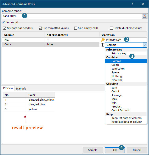
2. 고급 행 병합대화 상자에서 다음만 수행하면 됩니다:
- 결합하려는 범위를 선택합니다。
- 동일한 값을 포함하는 열을기본 키열로 설정합니다。
- 구분 기호을(를) 사용하여 셀을 결합합니다。
- 클릭하세요확인.
결과

Kutools for Excel– Excel 을 300 개 이상의 필수 도구로 강력하게 개선하여 작업을 더 빠르고 쉽게 처리하고, 스마트한 데이터 처리와 생산성을 위한 AI 기능을 활용하세요。지금 받기
- 이 기능에 대해 더 알아보려면 다음 문서를 참조하세요:Excel 에서 동일한 값을 빠르게 결합하거나 중복 행
VBA 코드를 사용하여 동일한 값이 있을 경우 셀 결합하기
다른 열에 동일한 값이 존재할 경우 VBA 코드를 사용하여 한 열의 셀을 결합할 수도 있습니다。
1. Alt+F11키를 눌러Microsoft Visual Basic 응용 프로그램창을 엽니다。
2. Microsoft Visual Basic 응용 프로그램창에서삽입>모듈을 클릭합니다。 그런 다음 아래 코드를 복사하여모듈창에 붙여넣습니다。
VBA 코드: 동일한 값이 있을 경우 셀 결합하기
Sub ConcatenateCellsIfSameValues()
	Dim xCol As New Collection
	Dim xSrc As Variant
	Dim xRes() As Variant
	Dim I As Long
	Dim J As Long
	Dim xRg As Range
	xSrc    = Range("A1", Cells(Rows.Count, "A").End(xlUp)).Resize(, 2)
	Set xRg = Range("D1")
	On Error Resume Next
	For I = 2 To UBound(xSrc)
		xCol.Add xSrc(I, 1), TypeName(xSrc(I, 1)) & CStr(xSrc(I, 1))
	Next I
	On Error GoTo 0
	ReDim xRes(1 To xCol.Count + 1, 1 To 2)
	xRes(1, 1) = "No"
	xRes(1, 2) = "Combined Color"
	For I = 1 To xCol.Count
		xRes(I + 1, 1) = xCol(I)
		For J = 2 To UBound(xSrc)
			If xSrc(J, 1) = xRes(I + 1, 1) Then
				xRes(I + 1, 2) = xRes(I + 1, 2) & ", " & xSrc(J, 2)
			End If
		Next J
		xRes(I + 1, 2) = Mid(xRes(I + 1, 2), 2)
	Next I
	Set xRg = xRg.Resize(UBound(xRes, 1), UBound(xRes, 2))
	xRg.NumberFormat = "@"
	xRg = xRes
	xRg.EntireColumn.AutoFit
End Sub
참고 사항:
3. F5키를 눌러 코드를 실행하면 제한된 범위에 결합된 결과가 표시됩니다。

데모: Kutools for Excel 을(를) 사용하여 동일한 값이 있을 경우 손쉽게 셀 결합하기
최고의 Office 생산성 도구
| 🤖 | KUTOOLS AI 도우미: 다음을 기반으로 데이터 분석 혁신하기:지능형 실행 | 코드 생성| 사용자 지정 수식 생성 | 데이터 분석 및 차트 생성| 향상된 함수 호출… |
| 인기 기능:찾기, 강조 표시 또는 중복 표시 | 빈 행 삭제 | 데이터 손실 없이 열 결합 또는 셀 제거 | 공식을 사용하지 않는 반올림... | |
| 슈퍼 LOOKUP:다중 조건 VLookup | 다중 값 VLookup | 여러 시트에서 VLookup | 퍼지 매치.... | |
| 고급 드롭다운 목록:드롭다운 목록 빠르게 생성 | 종속형 드롭다운 목록 | 다중 선택 드롭다운 목록.... | |
| 열 관리자:특정 수의 열 추가|열 이동|숨겨진 열의 표시 상태 전환|범위 및 열 비교... | |
| 주요 기능:그리드 포커스 | 디자인 보기 |향상된 수식 표시줄 | 워크북 및 시트 관리자 | 자원 라이브러리(자동 텍스트)| 날짜 선택기 | 워크시트 병합 | 암호화/셀 해독 | 목록으로 이메일 보내기 | 슈퍼 필터 | 특수 필터(굵은 글꼴이 있는 셀 필터링/기울임꼴/취소선。。。) 。。。 | |
| 상위 15 도구 모음:12 텍스트도구(텍스트 추가,특정 문자 삭제, ...)| 50+차트유형(간트 차트, ...)| 40+ 실용적인수식(생일을 기준으로 나이 계산, ...)| 19 삽입도구(QR 코드 삽입,경로에서 그림 삽입, ...)| 12 변환도구(단어로 변환하기,환율 변환, ...)| 7 병합 및 분할도구(고급 행 병합,셀 분할, ...)|그 외 더 많은 기능 |
Kutools for Excel 로 Excel 역량을 한 단계 업그레이드하고 전례 없는 효율성을 경험하세요。Kutools for Excel 는 생산성과 저장 시간을 향상시키는 300 개 이상의 고급 기능을 제공합니다。가장 필요한 기능을 지금 바로 확인하세요。。。
Office Tab 가 Office 에 탭 인터페이스를 제공하여 작업을 훨씬 쉽게 만들어 줍니다
- Word, Excel, PowerPoint 에서 탭 기반 편집 및 읽기 기능을 활성화합니다, Publisher, Access, Visio 및 Project 에서도 사용 가능합니다。
- 새 창이 아닌 동일한 창의 새 탭에서 여러 문서를 열고 생성할 수 있습니다。
- 50% 만큼 생산성을 높이고 매일 수백 번의 마우스 클릭을 줄여줍니다!
모든 Kutools 애드인。 하나의 설치 프로그램
Kutools for Office스위트 번들은 Excel, Word, Outlook 및 PowerPoint 용 애드인과 Office Tab Pro 를 포함하며, 다양한 Office 앱을 사용하는 팀에 이상적입니다。
- 올인원 스위트— Excel, Word, Outlook 및 PowerPoint 애드인 + Office Tab Pro
- 하나의 설치 프로그램, 하나의 라이선스— 몇 분 안에 설정 완료(MSI 지원)
- 함께 사용할수록 더 효과적입니다— Office 앱 전반에서 생산성 향상
- 30 일간 모든 기능 무료 체험— 등록이나 신용카드 필요 없음
- 최고의 가성비— 개별 애드인 구매 대비 절약