Excel에서 단일 셀에 여러 값을 반환하는 VLOOKUP 방법은 무엇입니까?
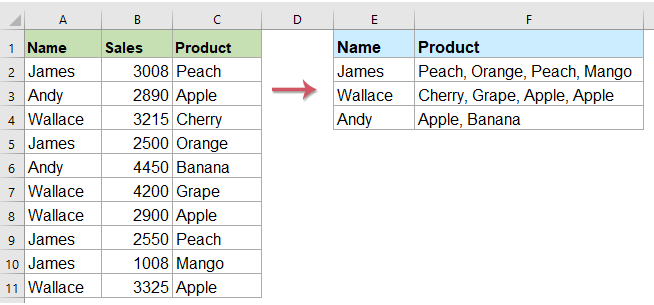
VLOOKUP은 Excel에서 강력한 기능이지만 기본적으로는 첫 번째 일치하는 값만 반환합니다. 모든 일치하는 값을 검색하여 하나의 셀에 결합해야 하는 경우는 어떨까요? 이는 데이터 세트를 분석하거나 정보를 요약할 때 일반적인 요구 사항입니다. 이 가이드에서는 수식과 유용한 기능을 사용하여 여러 값을 단일 셀에 반환하는 단계별 방법을 안내합니다.
TEXTJOIN 함수를 사용하여 여러 값을 하나의 셀로 반환 (Excel 2019 및 Office 365)
사용자 정의 함수를 사용하여 여러 값을 하나의 셀로 반환
TEXTJOIN 함수를 사용하여 여러 값을 하나의 셀로 반환 (Excel 2019 및 Office 365)
Excel 2019 및 Office 365와 같은 고급 버전의 Excel을 사용 중이라면, TEXTJOIN이라는 새로운 함수가 있습니다. 이 강력한 함수를 사용하면 빠르게 VLOOKUP을 실행하고 모든 일치하는 값을 하나의 셀로 반환할 수 있습니다.
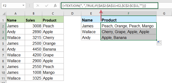
하나의 셀에 모든 일치하는 값을 반환
결과를 넣고 싶은 빈 셀에 아래 수식을 적용한 다음, 첫 번째 결과를 얻기 위해 Ctrl + Shift + Enter 키를 함께 누르고, 원하는 셀까지 채우기 핸들을 드래그하면 다음과 같은 스크린샷에 표시된 대로 모든 해당 값을 얻을 수 있습니다.
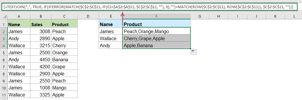
중복되지 않은 모든 일치하는 값을 하나의 셀로 반환
조회 데이터를 기반으로 중복되지 않은 모든 일치하는 값을 반환하려면 아래 수식이 도움이 될 수 있습니다.
다음 수식을 복사하여 빈 셀에 붙여넣고, 첫 번째 결과를 얻기 위해 Ctrl + Shift + Enter 키를 함께 누른 다음, 이 수식을 다른 셀에 복사하면 아래 스크린샷에 표시된 대로 중복되지 않은 모든 해당 값을 얻을 수 있습니다.
Kutools를 사용하여 여러 값을 하나의 셀로 반환
Kutools for Excel의 '고급 행 병합' 기능을 사용하면 복잡한 수식 없이도 여러 일치하는 값을 쉽게 검색하여 단일 셀로 결합할 수 있습니다! 수작업 방식을 잊고 Excel에서 더 효율적인 조회 작업 처리 방법을 발견하세요. Kutools for Excel이 이를 어떻게 가능하게 만드는지 살펴보겠습니다.
Kutools for Excel 설치 후에는 다음과 같이 하세요:
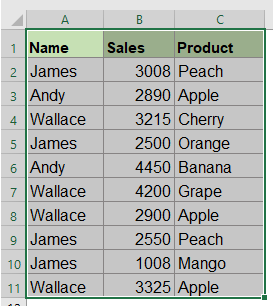
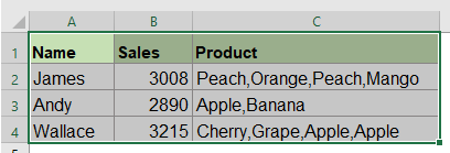
1. 다른 열을 기준으로 하나의 열 데이터를 결합하려는 데이터 범위를 선택하세요.
2. 'Kutools' > '병합 및 분할' > '고급 행 병합'을 클릭하세요. 스크린샷 참조:

3. 나타난 '고급 행 병합' 대화 상자에서:
- 결합할 기준 열 이름을 클릭한 다음 '주요 키'를 클릭하세요.
- 그런 다음 키 열을 기준으로 데이터를 결합하려는 다른 열을 클릭하고 '연산' 필드의 드롭다운 목록을 클릭하여 '결합' 섹션에서 결합된 데이터를 구분할 구분 기호를 선택하세요.
- 그런 다음 확인 버튼을 클릭하세요.

동일한 값에 따라 다른 열의 모든 해당 값이 단일 셀로 결합됩니다. 스크린샷 참조:
 |  |
팁: 셀을 병합하면서 중복 내용을 제거하려면 대화 상자의 '중복 값 삭제' 옵션을 선택하세요. 이렇게 하면 중복 항목 없이 고유한 항목만 결합되어 데이터가 더 깔끔하고 정리되며 추가 노력 없이도 관리가 용이해집니다. 스크린샷 참조:
 |  |
지금 바로 Kutools for Excel 다운로드 및 무료 평가판 시작!
사용자 정의 함수를 사용하여 여러 값을 하나의 셀로 반환
위의 TEXTJOIN 함수는 Excel 2019 및 Office 365에서만 사용할 수 있으며, 다른 낮은 버전의 Excel을 사용 중이라면 이 작업을 완료하기 위해 일부 코드를 사용해야 합니다.
하나의 셀에 모든 일치하는 값을 반환
1. 'ALT + F11' 키를 누르고 있으면 'Microsoft Visual Basic for Applications' 창이 열립니다.
2. '삽입' > '모듈'을 클릭하고 모듈 창에 다음 코드를 붙여넣으세요.
VBA 코드: 여러 값을 하나의 셀로 반환하는 Vlookup
Function ConcatenateIf(CriteriaRange As Range, Condition As Variant, ConcatenateRange As Range, Optional Separator As String = ",") As Variant
'Updateby Extendoffice
Dim xResult As String
On Error Resume Next
If CriteriaRange.Count <> ConcatenateRange.Count Then
    ConcatenateIf = CVErr(xlErrRef)
    Exit Function
End If
For i = 1 To CriteriaRange.Count
    If CriteriaRange.Cells(i).Value = Condition Then
        xResult = xResult & Separator & ConcatenateRange.Cells(i).Value
    End If
Next i
If xResult <> "" Then
    xResult = VBA.Mid(xResult, VBA.Len(Separator) + 1)
End If
ConcatenateIf = xResult
Exit Function
End Function
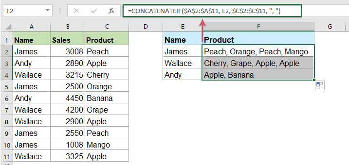
3. 그런 다음 코드를 저장하고 닫고, 워크시트로 돌아가서 결과를 배치하려는 특정 빈 셀에 =CONCATENATEIF($A$2:$A$11, E2, $C$2:$C$11, ", ") 수식을 입력한 다음 채우기 핸들을 아래로 드래그하여 원하는 모든 해당 값을 하나의 셀에 가져옵니다. 스크린샷 참조:
중복되지 않은 모든 일치하는 값을 하나의 셀로 반환
반환된 일치하는 값에서 중복을 무시하려면 아래 코드를 사용하세요.
1. 'Alt + F11' 키를 눌러 'Microsoft Visual Basic for Applications' 창을 엽니다.
2. '삽입' > '모듈'을 클릭하고 모듈 창에 다음 코드를 붙여넣으세요.
VBA 코드: 중복되지 않은 여러 일치하는 값을 하나의 셀로 반환하는 Vlookup
Function MultipleLookupNoRept(Lookupvalue As String, LookupRange As Range, ColumnNumber As Integer)
'Updateby Extendoffice
    Dim xDic As New Dictionary
    Dim xRows As Long
    Dim xStr As String
    Dim i As Long
    On Error Resume Next
    xRows = LookupRange.Rows.Count
    For i = 1 To xRows
        If LookupRange.Columns(1).Cells(i).Value = Lookupvalue Then
            xDic.Add LookupRange.Columns(ColumnNumber).Cells(i).Value, ""
        End If
    Next
    xStr = ""
    MultipleLookupNoRept = xStr
    If xDic.Count > 0 Then
        For i = 0 To xDic.Count - 1
            xStr = xStr & xDic.Keys(i) & ","
        Next
        MultipleLookupNoRept = Left(xStr, Len(xStr) - 1)
    End If
End Function
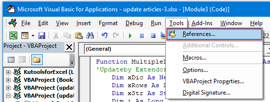
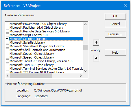
3. 코드를 삽입한 후 열린 'Microsoft Visual Basic for Applications' 창에서 '도구' > '참조'를 클릭하고, 나타난 '참조 - VBAProject' 대화 상자의 '사용 가능한 참조' 목록 상자에서 'Microsoft Scripting Runtime' 옵션을 선택하세요. 스크린샷 참조:
 |  |
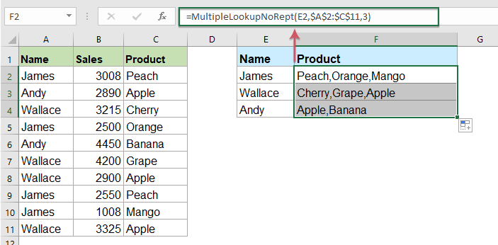
4. 그런 다음 대화 상자를 닫고 코드 창을 저장하고 닫은 후 워크시트로 돌아가서 결과를 출력하려는 빈 셀에 =MultipleLookupNoRept(E2,$A$2:$C$11,3) 수식을 입력하고 채우기 핸들을 아래로 드래그하여 모든 일치하는 값을 가져옵니다. 스크린샷 참조:
TEXTJOIN과 배열 함수를 결합한 수식을 사용하든, Kutools for Excel 또는 사용자 정의 함수와 같은 도구를 활용하든, 모든 접근 방식은 복잡한 조회 작업을 단순화하는 데 도움이 됩니다. 자신의 필요에 가장 적합한 방법을 선택하세요. 더 많은 Excel 팁과 트릭을 탐색하려는 경우 당사 웹사이트에서는 수천 개의 자습서를 제공합니다.
관련 기사 더 보기:
- VLOOKUP 함수의 몇 가지 기본 및 고급 예제
- Excel에서 VLOOKUP 함수는 대부분의 Excel 사용자에게 강력한 기능으로, 데이터 범위의 가장 왼쪽에서 값을 찾고 지정한 열에서 동일한 행의 일치하는 값을 반환합니다. 이 자습서에서는 Excel에서 VLOOKUP 함수를 사용하는 몇 가지 기본 및 고급 예제에 대해 설명합니다.
- 하나 이상의 기준에 따라 여러 일치하는 값을 반환
- 특정 값을 조회하고 일치하는 항목을 반환하는 것은 대부분의 사람들에게 VLOOKUP 함수를 사용하여 쉽습니다. 하지만 하나 이상의 기준에 따라 여러 일치하는 값을 반환해 본 적이 있습니까? 이 문서에서는 Excel에서 이 복잡한 작업을 해결하기 위한 몇 가지 수식을 소개합니다.
- Vlookup 및 여러 값을 세로로 반환
- 일반적으로 Vlookup 함수를 사용하여 첫 번째 해당 값을 얻을 수 있지만, 때로는 특정 기준에 따라 모든 일치하는 레코드를 반환하려고 합니다. 이 문서에서는 Vlookup을 수행하고 모든 일치하는 값을 세로, 가로 또는 하나의 셀로 반환하는 방법에 대해 설명합니다.
- 드롭다운 목록에서 여러 값을 Vlookup 및 반환
- Excel에서 드롭다운 목록에서 여러 해당 값을 Vlookup하고 반환하려면, 즉 드롭다운 목록에서 항목을 선택할 때 모든 관련 값이 한 번에 표시되도록 할 수 있는 방법은 무엇입니까? 이 문서에서는 단계별로 솔루션을 소개합니다.
최고의 오피스 생산성 도구
| 🤖 | Kutools AI 도우미: 데이터 분석에 혁신을 가져옵니다. 방법: 지능형 실행 | 코드 생성 | 사용자 정의 수식 생성 | 데이터 분석 및 차트 생성 | Kutools Functions 호출… |
| 인기 기능: 중복 찾기, 강조 또는 중복 표시 | 빈 행 삭제 | 데이터 손실 없이 열 또는 셀 병합 | 반올림(수식 없이) ... | |
| 슈퍼 LOOKUP: 다중 조건 VLOOKUP | 다중 값 VLOOKUP | 다중 시트 조회 | 퍼지 매치 .... | |
| 고급 드롭다운 목록: 드롭다운 목록 빠르게 생성 | 종속 드롭다운 목록 | 다중 선택 드롭다운 목록 .... | |
| 열 관리자: 지정한 수의 열 추가 | 열 이동 | 숨겨진 열의 표시 상태 전환 | 범위 및 열 비교 ... | |
| 추천 기능: 그리드 포커스 | 디자인 보기 | 향상된 수식 표시줄 | 통합 문서 & 시트 관리자 | 자동 텍스트 라이브러리 | 날짜 선택기 | 데이터 병합 | 셀 암호화/해독 | 목록으로 이메일 보내기 | 슈퍼 필터 | 특수 필터(굵게/이탤릭/취소선 필터 등) ... | |
| 15대 주요 도구 세트: 12 가지 텍스트 도구(텍스트 추가, 특정 문자 삭제, ...) | 50+ 종류의 차트(간트 차트, ...) | 40+ 실용적 수식(생일을 기반으로 나이 계산, ...) | 19 가지 삽입 도구(QR 코드 삽입, 경로에서 그림 삽입, ...) | 12 가지 변환 도구(단어로 변환하기, 통화 변환, ...) | 7 가지 병합 & 분할 도구(고급 행 병합, 셀 분할, ...) | ... 등 다양 |
Kutools for Excel과 함께 엑셀 능력을 한 단계 끌어 올리고, 이전에 없던 효율성을 경험하세요. Kutools for Excel은300개 이상의 고급 기능으로 생산성을 높이고 저장 시간을 단축합니다. 가장 필요한 기능을 바로 확인하려면 여기를 클릭하세요...
Office Tab은 Office에 탭 인터페이스를 제공하여 작업을 더욱 간편하게 만듭니다
- Word, Excel, PowerPoint에서 탭 편집 및 읽기를 활성화합니다.
- 새 창 대신 같은 창의 새로운 탭에서 여러 파일을 열고 생성할 수 있습니다.
- 생산성이50% 증가하며, 매일 수백 번의 마우스 클릭을 줄여줍니다!
모든 Kutools 추가 기능. 한 번에 설치
Kutools for Office 제품군은 Excel, Word, Outlook, PowerPoint용 추가 기능과 Office Tab Pro를 한 번에 제공하여 Office 앱을 활용하는 팀에 최적입니다.
- 올인원 제품군 — Excel, Word, Outlook, PowerPoint 추가 기능 + Office Tab Pro
- 설치 한 번, 라이선스 한 번 — 몇 분 만에 손쉽게 설정(MSI 지원)
- 함께 사용할 때 더욱 효율적 — Office 앱 간 생산성 향상
- 30일 모든 기능 사용 가능 — 회원가입/카드 불필요
- 최고의 가성비 — 개별 추가 기능 구매 대비 절약