텍스트 조건에 따라 Excel에서 값을 합산하는 방법은 무엇입니까?

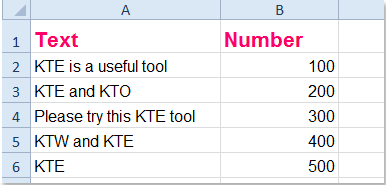
Excel에서 다른 열의 텍스트 조건에 따라 값을 합산해 본 적이 있습니까? 예를 들어, 다음과 같은 스크린샷에 표시된 워크시트에 데이터 범위가 있다고 가정해 보겠습니다. 이제 A열의 텍스트 값과 특정 기준을 충족하는 B열의 모든 숫자를 더하고 싶습니다. 예를 들어, A열의 셀에 KTE가 포함된 경우 숫자를 합산합니다.

특정 텍스트가 포함된 경우 다른 열에 따라 값을 합산 특정 텍스트로 시작하는 경우 다른 열에 따라 값을 합산 특정 텍스트로 끝나는 경우 다른 열에 따라 값을 합산 특정 텍스트만 있는 경우 다른 열에 따라 값을 합산

특정 텍스트가 포함된 경우 다른 열에 따라 값을 합산

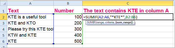
위의 데이터를 예로 들어, A열에 'KTE'라는 텍스트가 포함된 모든 값을 더하려면 다음 수식이 도움이 될 수 있습니다:

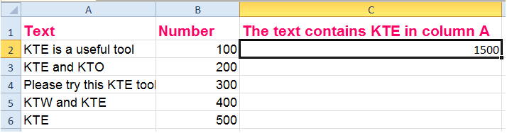
다음 수식 =SUMIF(A2:A6,"*KTE*",B2:B6)을 빈 셀에 입력하고 Enter 키를 누르세요. 그러면 A열에 해당하는 셀에 'KTE'라는 텍스트가 포함된 B열의 모든 숫자가 합산됩니다. 스크린샷을 참조하세요:

팁: 위의 수식에서 A2:A6은 값을 추가할 데이터 범위이며, *KTE*는 필요한 기준을 나타내고, B2:B6은 합산하려는 범위입니다.

Kutools AI로 엑셀의 마법을 풀다

• 스마트 실행: 셀 작업 수행, 데이터 분석 및 차트 생성 - 간단한 명령어로 모든 것을 처리합니다.
• 사용자 정의 수식: 작업을 간소화하기 위한 맞춤형 수식을 생성합니다.
• VBA 코딩: 손쉽게 VBA 코드를 작성하고 실행합니다.
• 수식 해석: 복잡한 수식도 쉽게 이해할 수 있습니다.
• 텍스트 번역: 스프레드시트 내 언어 장벽을 허물어 보세요.

AI 기반 도구로 엑셀 활용 능력을 강화하세요. 지금 다운로드하여 그 어느 때보다 높은 효율성을 경험해 보세요!

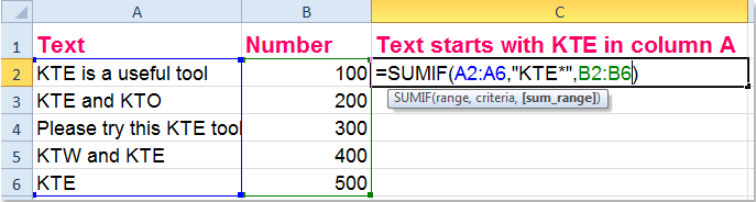
특정 텍스트로 시작하는 경우 다른 열에 따라 값을 합산

A열의 해당 셀 텍스트가 'KTE'로 시작하는 경우 B열의 셀 값을 합산하려면 이 수식을 적용할 수 있습니다: =SUMIF(A2:A6,"KTE*",B2:B6), 스크린샷을 참조하세요:

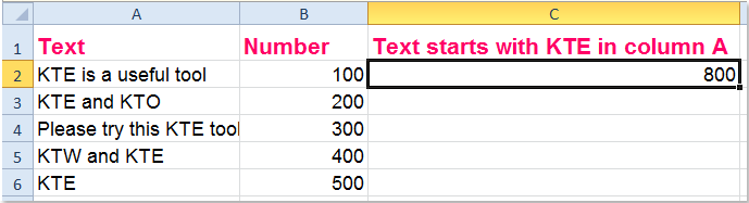팁: 위의 수식에서 A2:A6은 값을 추가할 데이터 범위이며, KTE*는 필요한 기준을 나타내고, B2:B6은 합산하려는 범위입니다.

특정 텍스트로 끝나는 경우 다른 열에 따라 값을 합산

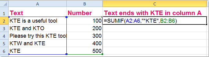
A열의 해당 셀 텍스트가 'KTE'로 끝나는 경우 B열의 모든 값을 합산하려면 이 수식이 도움이 될 수 있습니다: =SUMIF(A2:A6,"*KTE",B2:B6), (A2:A6은 값을 추가할 데이터 범위이며, KTE*는 필요한 기준을 나타내고, B2:B6은 합산하려는 범위) 스크린샷을 참조하세요:

특정 텍스트만 있는 경우 다른 열에 따라 값을 합산

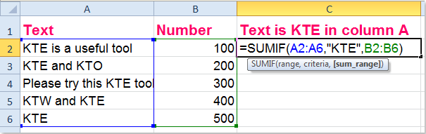
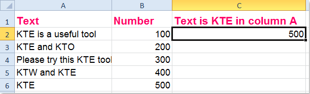
A열의 해당 셀 내용이 'KTE'인 경우 B열의 값을 합산하려면 다음 수식을 사용하세요: =SUMIF(A2:A6,"KTE",B2:B6), (A2:A6은 값을 추가할 데이터 범위이며, KTE는 필요한 기준을 나타내고, B2:B6은 합산하려는 범위) 그러면 A열에서 텍스트가 'KTE'인 경우에만 B열의 관련 숫자가 합산됩니다. 스크린샷을 참조하세요:

관련 문서:

Excel에서 매 n번째 행을 아래로 합산하는 방법은 무엇입니까?

Excel에서 텍스트와 숫자가 있는 셀을 합산하는 방법은 무엇입니까?