여러 열에서 고유한 값을 추출하는 방법은 무엇입니까?
Excel에서 여러 열에 걸쳐 데이터 세트를 자주 다룬다면, 동일한 열 내부 또는 다른 열 간에 특정 값이 중복되는 상황을 마주할 수 있습니다. 많은 보고서 작성이나 데이터 분석 작업에서는 전체 선택 영역에 걸쳐 단 한 번만 나타나는 모든 고유한 값을 식별하고 추출해야 하는 경우가 많습니다. 이를 수동으로 수행하면 시간이 많이 소요되고 오류가 발생하기 쉬우며, 특히 대규모 데이터 세트나 복잡한 표를 다룰 때 더욱 그렇습니다. 다행히도 Excel에서는 이러한 고유한 값을 효율적으로 추출하기 위한 다양한 방법을 제공합니다.
이 가이드에서는 사용자의 Excel 버전과 선호도에 따라 활용할 수 있는 몇 가지 솔루션을 소개합니다. 예를 들어, 모든 버전에 적합한 수식, 최신 버전용 동적 배열 수식, 간단한 결과를 위해 Kutools AI 도우미 사용, 시각적인 통합을 위해 피벗 테이블 사용, 복잡한 시나리오에서 자동화된 추출을 위한 VBA 코드 등입니다.
수식을 사용하여 여러 열에서 고유한 값 추출하기
때로는 기본 제공 Excel 기능을 사용하여 이러한 추출을 수행하고자 할 수 있습니다. 이 섹션에서는 두 가지 접근 방식을 사용하는 방법에 대해 설명합니다: 모든 Excel 버전에 적합한 배열 수식과 Excel 365 및 Excel 2021과 같은 최신 버전에서 사용 가능한 동적 배열 수식입니다. 이러한 방법은 직접적인 수식 기반 솔루션이 필요한 경우, 데이터 변경 시 자주 업데이트해야 하는 경우, 외부 추가 기능이나 코드를 피하려는 경우에 이상적입니다.
모든 Excel 버전에 대한 배열 수식을 사용하여 여러 열에서 고유한 값 추출하기
모든 Excel 버전에서의 호환성을 위해 배열 수식을 사용하면 동적 배열을 지원하지 않는 Excel에서도 여러 열에서 고유한 값을 추출할 수 있습니다. 이 접근 방식은 INDIRECT, TEXT, MIN, IF, COUNTIF, ROW 및 COLUMN 함수를 조합하여 사용하며, 다양한 데이터 구조에 유연하게 적용할 수 있습니다.
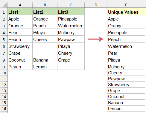
데이터가 A2:C9 범위에 있다고 가정합니다. E2 셀에서부터 고유한 값을 추출하려면 다음 절차를 따르세요:
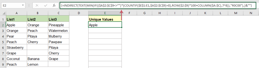
1. E2 셀(또는 출력 범위의 첫 번째 셀)을 클릭하고 다음 배열 수식을 입력하세요:
=INDIRECT(TEXT(MIN(IF(($A$2:$C$9<>"")*(COUNTIF($E$1:E1,$A$2:$C$9)=0),ROW($2:$9)*100+COLUMN($A:$C),7^8)),"R0C00"),)&""
- A2:C9는 고유한 값을 추출하려는 데이터 범위입니다.
- E1:E1은 첫 번째 출력 셀 바로 위의 셀을 참조하며, 이미 출력된 항목을 추적하는 데 필요합니다.
- $2:$9는 데이터의 행 참조이고, $A:$C는 열 참조입니다. 필요에 따라 워크시트 레이아웃에 맞게 조정하세요.
2. 수식을 입력한 후 Enter만 누르는 대신 Ctrl + Shift + Enter를 함께 눌러 배열 수식으로 확인하세요. 올바르게 수행되면 수식 표시줄에서 수식 주위에 중괄호 {}가 나타납니다. 그런 다음 E2에서 아래로 채우기 핸들을 드래그하세요. 빈 셀이 나타날 때까지 계속 드래그하면 더 이상 추출할 고유한 값이 없음을 나타냅니다. 이 과정을 통해 모든 고유한 값이 대상 열에 표시됩니다.

- $A$2:$C$9: 고유한 값을 검사할 전체 셀 집합을 지정합니다.
- IF(($A$2:$C$9<>"")*(COUNTIF($E$1:E1,$A$2:$C$9)=0), ROW($2:$9)*100+COLUMN($A:$C),7^8):
- $A$2:$C$9<>""는 빈 셀을 무시하도록 합니다.
- COUNTIF($E$1:E1,$A$2:$C$9)=0은 아직 추출되지 않은 새 값만 포함되도록 합니다.
- 두 조건이 모두 참인 경우 해당 출력은 셀의 행과 열 기반 계산으로 생성된 고유한 인덱스 번호입니다.
- 조건 중 하나라도 거짓인 경우 수식은 매우 큰 숫자(7^8)를 반환하여 우발적인 선택을 방지합니다.
- MIN(...): 가장 낮은 인덱스 번호를 식별하여 데이터 내에서 다음 사용 가능한 고유값의 위치를 효과적으로 찾습니다.
- TEXT(...,"R0C00"): R1C1 스타일을 사용하여 인덱스를 유효한 셀 참조로 변환합니다.
- INDIRECT(...): 위에서 생성된 셀 참조를 데이터 범위에서 값을 가져옵니다.
- &"": 수식 결과가 텍스트로 처리되도록 하여 서식 관련 문제를 방지합니다.
Excel 365, Excel 2021 및 이후 버전의 수식을 사용하여 여러 열에서 고유한 값 추출하기
Excel 365, Excel 2021 또는 이후 버전을 사용하는 경우 동적 배열 함수를 활용할 수 있으며, 이는 여러 열에서 고유한 값을 추출하는 더 간단하고 직관적인 방법을 제공합니다. UNIQUE와 TOCOL 함수를 사용하면 데이터를 여러 열에서 결합하고 중복을 한 번에 제거하는 것이 더 쉽고 빠릅니다 — 특히 지속적으로 업데이트되거나 대규모 데이터 세트를 다룰 때 유용합니다.
이 방법을 사용하려면 빈 셀(예: E2 또는 결과를 나타내고자 하는 곳)을 선택하고, 이 수식을 입력한 후 Enter를 누르세요:
=UNIQUE(TOCOL(A2:C9,1))Enter를 누른 후 A2:C9 범위의 모든 고유한 값이 수식 아래의 셀로 자동으로 표시됩니다. 이 기능은 특히 효율적이며, 원본 데이터가 변경될 때마다 출력이 동적으로 업데이트되어 수동으로 새로 고치는 단계를 줄여줍니다.

- TOCOL(A2:C9,1): 여러 열에 걸친 값 범위를 단일 열로 변환하고, 빈 셀을 자동으로 제거합니다.
- UNIQUE(...): 각 값을 한 번만 추출하여 깔끔하고 중복되지 않은 목록을 제공합니다.
Kutools AI 도우미를 사용하여 여러 열에서 고유한 값 추출하기
보다 간소화된 접근 방식을 원하거나 수작업을 줄이고 싶다면, Kutools for Excel의 Kutools AI 도우미를 사용하여 여러 열에서 고유한 값을 쉽게 추출할 수 있습니다. 이 방법은 수식에 익숙하지 않거나 수식 오류의 위험을 피하고 싶은 경우 특히 유용합니다. Kutools AI 도우미는 사용자의 지침을 해석하고 데이터를 자동으로 처리하여 초보자와 몇 번의 클릭으로 빠른 해결책을 찾고자 하는 사용자에게 이상적입니다.
설치 후 Kutools AI > AI 도우미를 클릭하여 "Kutools AI 도우미" 창을 엽니다:
- 채팅 상자에 요청 사항을 입력하세요. 예: "범위 A2:C9에서 고유한 값을 추출하고, 빈 셀을 무시하며, 결과를 E2에서 시작하도록 배치:"
- "보내기"를 클릭하거나 Enter를 누르세요. AI가 요청을 분석한 후 "실행"을 클릭하여 실행하세요. 결과는 즉시 표시되며, 사용자가 지정한 위치에 정확히 나타납니다.
팁: 이 솔루션은 데이터 추출 작업이 다양하거나 자연어 처리 기능을 원할 때 매우 유용합니다. 원본 데이터가 완벽하게 일관되지 않은 경우 빈 셀이 포함되었는지 또는 필터링되었는지 다시 확인하세요. 빈 항목은 AI 요청 세부 정보에 따라 포함되거나 필터링될 수 있습니다.

피벗 테이블을 사용하여 여러 열에서 고유한 값 추출하기
피벗 테이블은 고유한 값을 추출하는 또 다른 편리한 방법입니다. 특히 시각적 도구로 작업을 선호하고 고유 항목을 요약하거나 추가 분석(예: 발생 횟수 계산)을 원할 때 유용합니다. 이 접근 방식은 간단하고 수식이 필요 없습니다. 하지만 설정과 약간의 데이터 재배치가 필요하며, 특히 관련된 열이 서로 다른 제목을 가지고 있을 때 그렇습니다.
피벗 테이블을 사용하여 고유한 값을 추출하기 위한 권장 프로세스는 다음과 같습니다:
1. 데이터 왼쪽에 새 빈 열을 삽입합니다. 예를 들어 데이터가 B열에서 시작된다면 A열을 새로 삽입하세요. 이 조정은 올바른 범위 통합을 보장합니다.

2. 데이터 세트 내의 아무 셀을 선택하고 Alt + D를 누른 후 P를 빠르게 눌러 "피벗테이블 및 피벗차트 마법사"를 실행합니다. 마법사의 첫 번째 단계에서 "다중 통합 범위"를 선택하세요. 이를 통해 여러 열의 값을 단일 요약 필드로 결합할 수 있습니다.

3. 다음을 클릭하고 "나를 위한 단일 페이지 필드 만들기"를 선택하세요. 이 단계는 더 쉬운 고유값 추출을 위해 모든 데이터를 단일 그룹으로 정리합니다.

4. 다음 단계에서 전체 데이터 범위를 선택하고(새로운 빈 열 포함) "추가" 버튼을 클릭하여 선택 항목을 "모든 범위" 목록에 추가한 후 다음을 클릭하세요.

5. 마법사의 마지막 단계에서 피벗 테이블을 배치할 위치(새 워크시트 또는 기존 시트)를 선택하고 완료를 클릭하여 피벗 테이블 보고서를 생성하세요.

6. 새로운 피벗 테이블에서 "보고서에 추가할 필드 선택" 섹션의 모든 필드를 체크 해제하여 기본 보기 상태를 초기화합니다.

7. 마지막으로 "값" 필드를 행 영역으로 드래그하세요. 피벗 테이블은 원래의 다중 열 범위에서 모든 고유한 값을 정리된 단일 열로 표시합니다.

제한 사항: 데이터는 사전 준비가 필요하며, 원본 데이터 세트가 업데이트되면 고유값을 새로 확인하려면 피벗 테이블을 새로 고쳐야 합니다.
VBA 코드를 사용하여 여러 열에서 고유한 값 추출하기
자동화된 추출이 필요하거나 대규모 비정형 데이터 세트를 처리해야 하는 경우 VBA(Visual Basic for Applications) 코드를 사용하여 빠르고 재사용 가능한 솔루션을 제공할 수 있습니다. 이는 Excel VBA 에디터에 기본적인 지식을 가진 사용자나 수작업을 최소화하려는 반복 작업에 이상적입니다. VBA는 배열 수식보다 대규모 데이터를 더 효율적으로 처리할 수도 있습니다.
1. Alt + F11을 눌러 VBA 에디터를 엽니다. 나타나는 "Microsoft Visual Basic for Applications" 창에서 삽입 > 모듈을 클릭하여 새 모듈을 추가하세요.
2. 새 모듈에서 아래 코드를 붙여넣으세요:
VBA: 여러 열에서 고유한 값 추출하기
Sub Uniquedata()
'Updateby Extendoffice
Dim rng As Range
Dim InputRng As Range, OutRng As Range
Set dt = CreateObject("Scripting.Dictionary")
xTitleId = "KutoolsforExcel"
Set InputRng = Application.Selection
Set InputRng = Application.InputBox("Range :", xTitleId, InputRng.Address, Type:=8)
Set OutRng = Application.InputBox("Out put to (single cell):", xTitleId, Type:=8)
For Each rng In InputRng
    If rng.Value <> "" Then
        dt(rng.Value) = ""
    End If
Next
OutRng.Range("A1").Resize(dt.Count) = Application.WorksheetFunction.Transpose(dt.Keys)
End Sub
3. F5를 눌러 코드를 실행하세요. 데이터 범위를 선택하라는 대화 상자가 나타납니다. 관련된 모든 열(빈 셀이 포함된 열 포함)을 선택하세요.

4. 확인을 클릭하면 고유한 값을 출력할 위치를 묻는 메시지가 나타납니다. 결과를 나열하고자 하는 상단 셀(예: E2)을 지정하세요.

5. 확인을 클릭하면 매크로가 자동으로 실행됩니다. 모든 고유한 값이 지정된 위치에서부터 나타납니다.

- 수식을 사용할 때 #VALUE! 또는 #SPILL! 오류가 발생하면 범위를 확인하고 출력 영역이 비어 있는지 확인하세요.
- 데이터 범위 내의 숨겨진 행이나 병합된 셀을 항상 확인하세요. 이는 고유값 추출의 정확성에 영향을 미칠 수 있습니다.
- 배열 및 동적 배열 수식은 변경에 따라 자동으로 업데이트되지만, 고급 필터 및 피벗 테이블 솔루션은 수동으로 새로 고침하거나 다시 실행해야 할 수 있습니다.
- 반복 작업의 경우 일관성과 속도를 위해 VBA를 사용하여 추출을 자동화하는 것을 고려하세요.
- 복잡한 작업장, 특히 대량 추출이나 자동화 루틴을 적용하기 전에 데이터를 백업하세요.
관련 기사 더 보기:
- 목록에서 고유 및 고유한 값의 수 계산하기
- 중복 항목이 포함된 긴 목록이 있고 열 내에서 한 번만 나타나는 고유한 값의 수 또는 총 고유 값의 수를 계산하려는 경우가 있습니다. 이 문서에서는 Excel에서 고유 및 고유한 항목을 계산하는 효율적인 방법을 설명합니다.
- Excel에서 조건에 따라 고유한 값 추출하기
- 예를 들어, A 열의 특정 조건에 따라 B 열에서 고유한 이름만 추출하여 스크린샷과 같이 결과를 얻고자 한다고 가정합니다. 이 튜토리얼은 고유한 값을 추출할 때 조건을 적용하는 방법을 보여줍니다.
- Excel에서 고유한 값만 허용하기
- 워크시트 열에서 중복 값을 방지하고 고유한 항목만 허용하려는 경우 이 문서에서는 Excel에서 고유 규칙을 적용하는 실용적인 기술을 소개합니다.
- Excel에서 조건에 따라 고유한 값 합계 계산하기
- 예를 들어, 주문 열에서 고유한 값만 합계를 내고 인접한 열의 이름에 따라 조건을 두는 경우가 있습니다. 이 문서에서는 고유 및 조건부 계산을 결합하는 방법에 대해 논의합니다.
최고의 오피스 생산성 도구
| 🤖 | Kutools AI 도우미: 데이터 분석에 혁신을 가져옵니다. 방법: 지능형 실행 | 코드 생성 | 사용자 정의 수식 생성 | 데이터 분석 및 차트 생성 | Kutools Functions 호출… |
| 인기 기능: 중복 찾기, 강조 또는 중복 표시 | 빈 행 삭제 | 데이터 손실 없이 열 또는 셀 병합 | 반올림(수식 없이) ... | |
| 슈퍼 LOOKUP: 다중 조건 VLOOKUP | 다중 값 VLOOKUP | 다중 시트 조회 | 퍼지 매치 .... | |
| 고급 드롭다운 목록: 드롭다운 목록 빠르게 생성 | 종속 드롭다운 목록 | 다중 선택 드롭다운 목록 .... | |
| 열 관리자: 지정한 수의 열 추가 | 열 이동 | 숨겨진 열의 표시 상태 전환 | 범위 및 열 비교 ... | |
| 추천 기능: 그리드 포커스 | 디자인 보기 | 향상된 수식 표시줄 | 통합 문서 & 시트 관리자 | 자동 텍스트 라이브러리 | 날짜 선택기 | 데이터 병합 | 셀 암호화/해독 | 목록으로 이메일 보내기 | 슈퍼 필터 | 특수 필터(굵게/이탤릭/취소선 필터 등) ... | |
| 15대 주요 도구 세트: 12 가지 텍스트 도구(텍스트 추가, 특정 문자 삭제, ...) | 50+ 종류의 차트(간트 차트, ...) | 40+ 실용적 수식(생일을 기반으로 나이 계산, ...) | 19 가지 삽입 도구(QR 코드 삽입, 경로에서 그림 삽입, ...) | 12 가지 변환 도구(단어로 변환하기, 통화 변환, ...) | 7 가지 병합 & 분할 도구(고급 행 병합, 셀 분할, ...) | ... 등 다양 |
Kutools for Excel과 함께 엑셀 능력을 한 단계 끌어 올리고, 이전에 없던 효율성을 경험하세요. Kutools for Excel은300개 이상의 고급 기능으로 생산성을 높이고 저장 시간을 단축합니다. 가장 필요한 기능을 바로 확인하려면 여기를 클릭하세요...
Office Tab은 Office에 탭 인터페이스를 제공하여 작업을 더욱 간편하게 만듭니다
- Word, Excel, PowerPoint에서 탭 편집 및 읽기를 활성화합니다.
- 새 창 대신 같은 창의 새로운 탭에서 여러 파일을 열고 생성할 수 있습니다.
- 생산성이50% 증가하며, 매일 수백 번의 마우스 클릭을 줄여줍니다!
모든 Kutools 추가 기능. 한 번에 설치
Kutools for Office 제품군은 Excel, Word, Outlook, PowerPoint용 추가 기능과 Office Tab Pro를 한 번에 제공하여 Office 앱을 활용하는 팀에 최적입니다.
- 올인원 제품군 — Excel, Word, Outlook, PowerPoint 추가 기능 + Office Tab Pro
- 설치 한 번, 라이선스 한 번 — 몇 분 만에 손쉽게 설정(MSI 지원)
- 함께 사용할 때 더욱 효율적 — Office 앱 간 생산성 향상
- 30일 모든 기능 사용 가능 — 회원가입/카드 불필요
- 최고의 가성비 — 개별 추가 기능 구매 대비 절약