Excel에서 새 데이터를 입력한 후 차트를 자동으로 업데이트하려면 어떻게 해야 하나요?
매일의 판매 데이터를 시각적으로 추적하기 위해 Excel에서 차트를 생성했다고 가정해 봅시다. 그리고 새로운 판매 기록이 추가될 때마다 이 데이터를 정기적으로 업데이트합니다. 일반적으로 범위 내에서 데이터를 삽입하거나 수정할 때마다 차트가 최신 정보를 표시하도록 차트의 데이터 범위를 수동으로 조정해야 할 수 있습니다. 이러한 수동 작업은 특히 대량의 데이터셋이나 자주 변경되는 정보에서는 반복적이고 오류가 발생하기 쉬워질 수 있습니다. 다행히도, 새 데이터가 추가되었을 때 차트를 자동으로 업데이트하는 실용적인 방법들이 있어 대시보드나 보고서를 일관되게 최신 상태로 유지할 수 있게 도와줍니다.
이러한 자동 차트 업데이트를 Excel에서 수행하는 방법에는 여러 가지가 있으며, 각각은 다양한 Excel 버전과 데이터 구조에 맞춰져 있습니다. 아래에서 설명된 솔루션은 데이터를 Excel 테이블로 변환하는 방법, 동적 수식을 사용하여 이름이 지정된 범위를 활용하는 방법, 그리고 복잡하거나 사용자 정의 요구 사항에 특히 유용한 VBA 매크로를 적용하는 방법을 포함합니다.
새 데이터 입력 후 테이블 생성으로 차트 자동 업데이트
새 데이터 입력 후 동적 수식을 사용하여 차트 자동 업데이트
새 데이터 입력 후 VBA 코드를 사용하여 차트 자동 업데이트
 새 데이터 입력 후 테이블 생성으로 차트 자동 업데이트
연속적인 데이터 범위와 해당 열 차트가 있는 경우, 데이터 범위를 Excel 테이블로 변환함으로써 새 정보를 추가할 때 차트가 즉시 업데이트되도록 할 수 있습니다. 이 방법은 Excel 2007 이상에서 사용 가능하며, 확장 가능한 데이터셋 관리를 훨씬 쉽게 만들어 줍니다. 주요 장점은 테이블을 참조하는 차트가 테이블에 추가된 새 행을 자동으로 포함한다는 것입니다. 다음은 이를 수행하는 방법입니다:

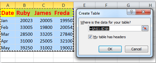
1. 헤더와 일일 값이 모두 포함된 기존 데이터 범위를 선택하세요. 그런 다음 삽입 탭으로 이동하여 표를 클릭하세요. 스크린샷을 참조하세요:

2. 표 만들기 대화 상자에서 데이터에 헤더가 포함되어 있다면 내 표에 머리글이 있음 옵션이 선택되어 있는지 확인하고 확인을 클릭하세요. (범위에 헤더가 없는 경우 이 상자를 선택하지 않은 채로 두세요.)
3. 이제 선택한 데이터 범위는 구조화된 Excel 표로 형식이 지정됩니다. 아래와 같이 표 스타일 형식이 자동으로 적용된 것을 확인할 수 있습니다:

4. 이제 테이블의 마지막 행 바로 아래에 새 행을 추가하면(예: 6월 데이터 입력) 테이블과 연결된 차트가 자동으로 확장되어 추가 단계 없이 최신 데이터를 표시합니다. 참고용 예제는 다음과 같습니다:

참고 및 실용 팁:
1. 새로 입력된 데이터는 반드시 직접 인접해야 합니다. 즉, 새 데이터와 기존 데이터 사이에 빈 행이나 열이 있어서는 안 되며, 그렇지 않으면 테이블(및 차트)이 확장을 인식하지 못합니다.
2. 테이블 내 어디든 새 행을 삽입할 수 있습니다. 차트는 자동으로 업데이트되며, 이는 과거 기록을 업데이트하는 데에도 유용합니다.
3. 차트가 예상대로 업데이트되지 않는다면 차트의 소스 데이터 범위가 정적 범위가 아닌 테이블을 참조하고 있는지 확인하세요.

Kutools AI로 엑셀의 마법을 풀다
- 스마트 실행: 셀 작업 수행, 데이터 분석 및 차트 생성 - 간단한 명령어로 모든 것을 처리합니다.
- 사용자 정의 수식: 작업을 간소화하기 위한 맞춤형 수식을 생성합니다.
- VBA 코딩: 손쉽게 VBA 코드를 작성하고 실행합니다.
- 수식 해석: 복잡한 수식도 쉽게 이해할 수 있습니다.
- 텍스트 번역: 스프레드시트 내 언어 장벽을 허물어 보세요.
새 데이터 입력 후 동적 수식을 사용하여 차트 자동 업데이트
데이터를 Excel 표로 변환하고 싶지 않다면, 수식으로 동작하는 동적 이름이 지정된 범위를 사용할 수 있습니다. 이 방법은 OFFSET과 COUNTA 함수를 활용하여 현재 존재하는 데이터 양에 따라 자동으로 크기가 조절되는 범위를 정의합니다. 이 접근 방식은 데이터 구조가 고정되어 있지만 항목이 자주 추가되거나 제거될 때 특히 유용합니다. 아래의 실용적인 단계를 참조하세요:

1. 먼저 각 데이터 열에 대해 동적 이름이 지정된 범위를 정의하세요. 수식 탭으로 이동하여 이름 정의를 클릭하세요.
2. 새 이름 대화 상자에서 적절한 이름을 입력합니다(예: 날짜 열의 경우 Date). Scope에서 올바른 워크시트를 선택하고 Refers to 필드에 동적 수식을 입력합니다. 예: =OFFSET($A$2,0,0,COUNTA($A:$A)-1). 스크린샷을 참조하세요:

3. 확인을 클릭하여 저장하세요. 관련된 모든 시리즈 또는 데이터 열에 대해 위의 단계를 반복하세요. 다음 수식들을 사용합니다:
- B열: Ruby: =OFFSET($B$2,0,0,COUNTA($B:$B)-1);
- C열: James: =OFFSET($C$2,0,0,COUNTA($C:$C)-1);
- D열: Freda: =OFFSET($D$2,0,0,COUNTA($D:$D)-1)
이 동적 이름이 지정된 범위들은 각 열에 새 데이터가 추가되면 범위가 자동으로 확장되거나 축소되도록 보장합니다. OFFSET 수식은 첫 번째 데이터 행부터 시작하며, COUNTA는 지정된 열의 비어있지 않은 셀의 총 수에 따라 범위 크기를 조정합니다.
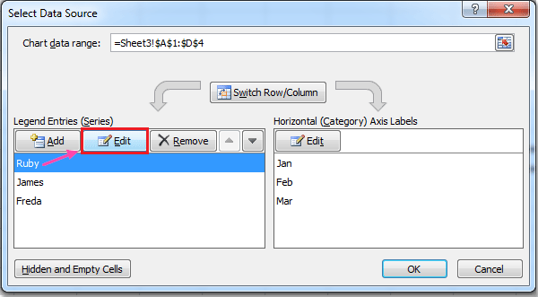
4. 모든 이름이 지정된 범위를 정의한 후, 연결된 차트의 열 중 하나를 마우스 오른쪽 버튼으로 클릭하고 컨텍스트 메뉴에서 데이터 선택을 선택하세요.

5. 데이터 원본 선택 대화 상자에서 관련된 시리즈(예: Ruby)를 강조 표시하고 편집을 클릭한 후 Series values로 적절한 동적 범위를 입력하세요(예: =Sheet3!Ruby). 아래를 참조하세요:
 |
 |
6. 추가 시리즈 각각에 대해 해당하는 동적 이름이 지정된 범위를 참조하여 반복합니다:
- James: Series values: =Sheet3!James;
- Freda: Series values: =Sheet3!Freda
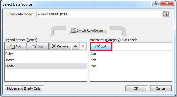
7. 가로(범주) 축 레이블의 경우, 가로(범주) 축 레이블 아래의 편집을 클릭하고 날짜 열에 대한 동적 범위 이름을 제공하세요.
 |
 |
8. 확인을 클릭하여 모든 대화 상자를 확인하고 종료하세요. 이제부터 워크시트에 새 데이터 항목을 계속 추가하면 차트는 최신 데이터 포인트를 반영하여 자동으로 업데이트됩니다.

- 1. 데이터는 열의 연속된 셀에 입력되어야 합니다. 동적 수식은 행 간 간격을 처리하지 않습니다. 행을 건너뛰면 자동 확장이 의도한 대로 작동하지 않을 수 있습니다.
- 2. 이 방법은 새 헤더가 추가되었을 때 추가 시리즈나 열을 인식하지 못합니다. 새 이름이 지정된 범위를 생성하고 차트 데이터 원본을 그에 따라 업데이트해야 합니다.
- 3. 동적 범위가 확장되지 않으면 COUNTA 범위를 다시 확인하고 의도한 데이터 아래에 불필요한 항목이 없는지 확인하세요.
- 4. 워크시트 이름이나 셀 위치를 변경하면 동적 동작을 유지하기 위해 이름이 지정된 범위 참조를 업데이트해야 합니다.
새 데이터 입력 후 VBA 코드를 사용하여 차트 자동 업데이트
비연속적인 데이터를 처리하거나 완전히 새로운 데이터 시리즈를 자동으로 감지하거나 여러 차트를 동시에 업데이트하는 등 고급 요구 사항의 경우, VBA 매크로는 더 큰 유연성과 자동화를 제공할 수 있습니다. 데이터 변경에 반응하는 짧은 매크로를 작성하여 차트의 데이터 소스를 새로 고치는 과정을 자동화할 수 있으며, 이전 방법들로는 직접적으로 다룰 수 없는 더 복잡한 시나리오에 대응할 수 있습니다.
데이터가 퍼져 있거나 규칙적인 블록이 아니거나 차트에 새 시리즈나 열을 자주 추가하는 경우 이 솔루션을 권장합니다. 다음 단계에 따라 설정하세요:
1. 먼저 차트를 평소처럼 삽입하세요.
2. Alt + F11을 눌러 VBA 편집기를 엽니다.
3. VBA 편집기에서 삽입 > 모듈을 클릭하여 새 코드 모듈을 삽입하세요. 그런 다음 다음 매크로 코드를 모듈 창에 입력하세요:
Sub AutoUpdateChartData()
    Dim ws As Worksheet
    Dim chrt As ChartObject
    Dim lastRow As Long

    On Error Resume Next
    xTitleId = "KutoolsforExcel"

    Set ws = ActiveSheet
    Set chrt = ws.ChartObjects(1) ' Modify if you have more than 1 chart on the sheet

    ' Find the last row of data in column A (assume your data starts from A1, adjust as needed)
    lastRow = ws.Cells(ws.Rows.Count, "A").End(xlUp).Row

    ' Set the data range for the chart dynamically (Modify range as per your data location)
    chrt.Chart.SetSourceData Source:=ws.Range("A1:D" & lastRow)

    On Error GoTo 0
End Sub3. 매크로를 실행하려면 실행 버튼을 클릭하세요. 이제 차트는 마지막으로 채워진 행까지 모든 현재 데이터를 즉시 업데이트합니다.
향상된 자동화를 위해 새 데이터가 입력될 때마다 이 매크로가 자동으로 트리거되도록 설정할 수 있습니다.
이를 적용하려면 워크시트 탭을 마우스 오른쪽 버튼으로 클릭하고 코드 보기 선택 후 위의 코드를 워크시트 모듈에 붙여넣으세요. 이제 시트에 변경 사항이 있을 때마다 매크로가 실행되어 차트가 항상 최신 상태를 유지합니다.
Private Sub Worksheet_Change(ByVal Target As Range)
    On Error Resume Next
    xTitleId = "KutoolsforExcel"
    Call AutoUpdateChartData
End Sub
팁 및 참고:
- 데이터 범위(예: "A1:D" & lastRow)는 실제 데이터 세트의 위치와 구조에 맞게 수정해야 합니다. 비연속적인 범위의 경우 코드에서 직접 범위 문자열을 사용자 정의하는 것이 좋습니다.
- 여러 개의 차트가 있는 경우 ChartObjects(1)을 올바른 차트를 참조하도록 수정하거나 필요에 따라 워크시트의 모든 ChartObjects를 반복해야 할 수 있습니다.
- 이 VBA 솔루션은 동적이고 복잡한 데이터 세트에 최대의 유연성을 제공하지만 매크로를 활성화하고 파일을 매크로 사용이 가능한 통합 문서(.xlsm)로 저장해야 합니다.
- 차트가 예상대로 업데이트되지 않는 경우 매크로의 소스 데이터 범위가 실제 데이터 블록과 일치하는지 확인하고 Excel 환경에서 매크로가 활성화되어 있는지 확인하세요.
관련 기사:
Excel에서 차트에 가로 평균선을 추가하려면 어떻게 해야 하나요?
Excel에서 조합 차트를 생성하고 이에 대한 보조 축을 추가하려면 어떻게 해야 하나요?
최고의 오피스 생산성 도구
| 🤖 | Kutools AI 도우미: 데이터 분석에 혁신을 가져옵니다. 방법: 지능형 실행 | 코드 생성 | 사용자 정의 수식 생성 | 데이터 분석 및 차트 생성 | Kutools Functions 호출… |
| 인기 기능: 중복 찾기, 강조 또는 중복 표시 | 빈 행 삭제 | 데이터 손실 없이 열 또는 셀 병합 | 반올림(수식 없이) ... | |
| 슈퍼 LOOKUP: 다중 조건 VLOOKUP | 다중 값 VLOOKUP | 다중 시트 조회 | 퍼지 매치 .... | |
| 고급 드롭다운 목록: 드롭다운 목록 빠르게 생성 | 종속 드롭다운 목록 | 다중 선택 드롭다운 목록 .... | |
| 열 관리자: 지정한 수의 열 추가 | 열 이동 | 숨겨진 열의 표시 상태 전환 | 범위 및 열 비교 ... | |
| 추천 기능: 그리드 포커스 | 디자인 보기 | 향상된 수식 표시줄 | 통합 문서 & 시트 관리자 | 자동 텍스트 라이브러리 | 날짜 선택기 | 데이터 병합 | 셀 암호화/해독 | 목록으로 이메일 보내기 | 슈퍼 필터 | 특수 필터(굵게/이탤릭/취소선 필터 등) ... | |
| 15대 주요 도구 세트: 12 가지 텍스트 도구(텍스트 추가, 특정 문자 삭제, ...) | 50+ 종류의 차트(간트 차트, ...) | 40+ 실용적 수식(생일을 기반으로 나이 계산, ...) | 19 가지 삽입 도구(QR 코드 삽입, 경로에서 그림 삽입, ...) | 12 가지 변환 도구(단어로 변환하기, 통화 변환, ...) | 7 가지 병합 & 분할 도구(고급 행 병합, 셀 분할, ...) | ... 등 다양 |
Kutools for Excel과 함께 엑셀 능력을 한 단계 끌어 올리고, 이전에 없던 효율성을 경험하세요. Kutools for Excel은300개 이상의 고급 기능으로 생산성을 높이고 저장 시간을 단축합니다. 가장 필요한 기능을 바로 확인하려면 여기를 클릭하세요...
Office Tab은 Office에 탭 인터페이스를 제공하여 작업을 더욱 간편하게 만듭니다
- Word, Excel, PowerPoint에서 탭 편집 및 읽기를 활성화합니다.
- 새 창 대신 같은 창의 새로운 탭에서 여러 파일을 열고 생성할 수 있습니다.
- 생산성이50% 증가하며, 매일 수백 번의 마우스 클릭을 줄여줍니다!
모든 Kutools 추가 기능. 한 번에 설치
Kutools for Office 제품군은 Excel, Word, Outlook, PowerPoint용 추가 기능과 Office Tab Pro를 한 번에 제공하여 Office 앱을 활용하는 팀에 최적입니다.
- 올인원 제품군 — Excel, Word, Outlook, PowerPoint 추가 기능 + Office Tab Pro
- 설치 한 번, 라이선스 한 번 — 몇 분 만에 손쉽게 설정(MSI 지원)
- 함께 사용할 때 더욱 효율적 — Office 앱 간 생산성 향상
- 30일 모든 기능 사용 가능 — 회원가입/카드 불필요
- 최고의 가성비 — 개별 추가 기능 구매 대비 절약